Franck–Hertz Experiment

The Franck–Hertz experiment is a collision experiment showing that atoms can absorb kinetic energy from electrons only at discrete excitation thresholds. It gave a direct, non-spectroscopic route to atomic energy levels: the evidence came from electron energy loss in mercury vapor, not from first looking at emitted line spectra.

The result belongs beside the Bohr Model and Line Spectra. Spectroscopy showed that atoms emit and absorb sharply defined frequencies. Franck and Hertz showed that electron impacts also encounter sharply defined internal energy gaps.

Why This Experiment Matters

By 1913, Bohr’s hydrogen model had made quantized stationary states a compelling way to understand spectral lines. But line spectra alone could still be read as facts about radiation frequencies. The Franck–Hertz experiment made the same discreteness appear in collisions.

Its central lesson is:

$$\text{an atom changes internal state only when the transferred energy matches an allowed gap.}$$

For mercury vapor the first strong threshold is about

$$\Delta E\simeq 4.9\,\mathrm{eV}.$$

That energy corresponds to ultraviolet radiation with wavelength

$$\lambda = \frac{hc}{\Delta E} \simeq 254\,\mathrm{nm},$$

close to the mercury resonance line. The collision threshold and the spectral line are therefore two faces of the same energy-level structure.

Electron-Atom Collision Setup

In the usual Franck–Hertz tube, a heated cathode emits electrons. An accelerating voltage $V$ gives the electrons kinetic energy as they move through a low-pressure gas, historically mercury vapor. A small retarding potential near the collector allows only electrons with enough remaining kinetic energy to reach the collector and contribute to the measured current.

The measured observable is the collector current $I$ as a function of the accelerating voltage $V$.

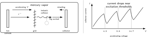
The Franck–Hertz experiment compares electron transport through mercury vapor with an accelerating voltage. When electrons reach the excitation energy, inelastic collisions remove about $4.9\,\mathrm{eV}$ from their kinetic energy, producing drops in collector current.

Below threshold, electron-atom collisions are mostly elastic on the energy scale relevant here. The electrons may change direction, but they do not lose a fixed large amount of kinetic energy to atomic excitation. The current generally rises as $V$ increases because more electrons reach the collector.

At the threshold, a new inelastic channel opens. Electrons can excite mercury atoms and lose approximately $\Delta E$ in a collision. Many of those electrons then fail to overcome the retarding field, so the collector current drops.

Energy Loss at Discrete Thresholds

The elementary energy estimate is

$$K_{\mathrm{electron}} \simeq eV,$$

up to apparatus-dependent corrections such as contact potentials and the electron energy distribution. An inelastic excitation becomes possible when

$$eV \gtrsim E_n-E_0,$$

where $E_0$ is the atomic ground-state energy and $E_n$ is an excited-state energy.

For the first strong mercury excitation,

$$e\Delta V \simeq 4.9\,\mathrm{eV}.$$

As the accelerating voltage is increased further, electrons can gain enough energy for one excitation, accelerate again, and later undergo another excitation. This produces repeated current minima separated approximately by the excitation potential:

$$\Delta V \simeq 4.9\,\mathrm{V} \quad \text{for mercury in the idealized textbook pattern.}$$

The repeated spacing is more important than any single perfectly sharp minimum. Real tubes have finite gas pressure, nonzero temperature, contact potentials, space-charge effects, and a distribution of collision locations.

Relation to Spectral Lines

If a mercury atom is excited by electron impact, it later returns toward lower energy states by radiative or nonradiative processes. For a radiative transition with photon frequency $\nu$,

$$h\nu = E_n-E_m.$$

The collision threshold measures the left side of the same energy-gap structure from a different direction:

$$\text{electron energy loss} \quad \longleftrightarrow \quad \text{atomic excitation energy} \quad \longleftrightarrow \quad \text{possible emitted photon energy}.$$

This is why the experiment was so historically persuasive. It tied atomic spectra to mechanical energy transfer in electron collisions. The same discrete energies appeared whether one watched light emitted by atoms or measured the energy lost by electrons.

Why This Supports Quantized Levels

A classical atom with continuously variable internal energy would not naturally predict repeated, atom-specific current drops at well-defined voltages. One could imagine continuous excitation, heating, or complicated collision losses, but the sharp threshold pattern calls for allowed and forbidden internal energy changes.

The quantum interpretation is that the atom has stationary states with discrete energies:

$$H_{\mathrm{atom}}\lvert n\rangle = E_n\lvert n\rangle.$$

An electron can transfer energy to the atom if the collision has enough available kinetic energy and the relevant transition is dynamically allowed. The threshold condition is energy conservation:

$$K_{\mathrm{in}} \ge K_{\mathrm{out}} + E_n-E_0.$$

At threshold, $K_{\mathrm{out}}$ can become too small for the electron to reach the collector, explaining the current minimum.

Modern Interpretation

In modern language, the experiment is an inelastic scattering problem. The incoming electron and the atom form an initial scattering channel,

$$\lvert \mathbf{k},0\rangle,$$

and an allowed inelastic outcome has the atom excited:

$$\lvert \mathbf{k}',n\rangle.$$

Energy conservation requires

$$\frac{\hbar^2 k^2}{2m_e}+E_0 = \frac{\hbar^2 k'^2}{2m_e}+E_n,$$

so the final electron momentum is real only when the incoming kinetic energy exceeds the excitation gap. Transition probabilities depend on the electron-atom interaction, selection rules, collision energy, and experimental geometry. The current-voltage curve is therefore not a direct drawing of the atom’s spectrum; it is a transport measurement whose threshold positions reveal excitation energies.

The clean pedagogical formula,

$$e\Delta V\simeq E_n-E_0,$$

is a threshold estimate. Precision interpretation must account for contact potentials, the work function of the electrodes, gas pressure, mean free path, retarding voltage, and the fact that electrons do not all collide at the same place with the same kinetic energy.

Historical Caution

The experiment is often described as a simple confirmation of the Bohr model. That is too tidy.

Franck and Hertz’s 1914 work was part of an evolving vocabulary of excitation, ionization, and resonance radiation. The result supported the emerging idea of discrete atomic internal energies, and it became especially clear in hindsight after the old quantum theory and spectroscopy were placed into a broader quantum framework. It did not observe Bohr orbits, did not derive the Schrödinger equation, and did not by itself determine atomic wavefunctions.

The historically careful statement is: the Franck–Hertz experiment gave direct evidence that atoms have discrete excitation energies accessible through electron impact.

What the Experiment Does Not Prove by Itself

• It does not show literal electron orbits.
• It does not prove the whole Bohr model.
• It does not derive Hilbert space, operators, or the Born rule.
• It does not imply every collision above threshold is inelastic.
• It does not make the measured voltage spacing identical to an atomic energy gap without apparatus corrections.
• It does not replace spectroscopy; it corroborates the energy-level interpretation from another experimental angle.

Common Mistakes

• Calling $4.9\,\mathrm{eV}$ the ionization energy of mercury. It is an excitation energy; mercury ionization requires a larger energy.
• Saying the electrons vanish at a current drop. They mostly lose kinetic energy in inelastic collisions and fail to reach the collector.
• Treating the current minima as perfectly located at exact integer multiples of $4.9\,\mathrm{V}$ in every apparatus.
• Forgetting the retarding potential. The current drop is visible because post-collision electrons may no longer have enough energy to pass the collector barrier.
• Saying the experiment measured spectral lines directly. It measured electron current; spectral emission supplies the complementary evidence.
• Retelling the experiment as if modern stationary-state notation was already the original language of the 1914 papers.

Cross-Links

• Atomic Structure and Spectra
• Line Spectra
• Rydberg Formula
• Bohr Model
• Energy Eigenstates
• Spectra
• Transition Probabilities
• Hamiltonians
• Atomic Spectra Reference
• Franck–Hertz Experiment Reference
• AMO Experiment Index
• Evidence Map

References

• J. Franck and G. Hertz, “Ueber Zusammenstoesse zwischen Elektronen und Molekuelen des Quecksilberdampfes und die Ionisierungsspannung desselben,” Verhandlungen der Deutschen Physikalischen Gesellschaft 16, 457-467, 1914.
• J. Franck and G. Hertz, “Ueber die Erregung der Quecksilberresonanzlinie 253.6 nm durch Elektronenstoesse,” Verhandlungen der Deutschen Physikalischen Gesellschaft 16, 512-517, 1914.
• Nobel Prize Outreach, The Nobel Prize in Physics 1925.
• J. Franck, Transformations of kinetic energy of free electrons into excitation energy of atoms by impacts, Nobel Lecture, 1926.
• M. Jammer, The Conceptual Development of Quantum Mechanics, 2nd ed., American Institute of Physics, 1989.
• H. Haken and H. C. Wolf, The Physics of Atoms and Quanta, 7th ed., Springer, 2005.
• B. H. Bransden and C. J. Joachain, Physics of Atoms and Molecules, 2nd ed., Pearson, 2003.

Exercises

1. A Franck–Hertz tube using mercury shows adjacent current minima separated by about $4.9\,\mathrm{V}$. Estimate the corresponding excitation energy in electronvolts.

Solution

An electron accelerated through a voltage difference $\Delta V$ gains energy $e\Delta V$. In electronvolt units, $1\,\mathrm{V}$ corresponds to $1\,\mathrm{eV}$ for an electron charge magnitude. Thus

$$\Delta E\simeq e\Delta V\simeq 4.9\,\mathrm{eV}.$$

2. Use $\lambda=hc/\Delta E$ and $hc\simeq 1240\,\mathrm{eV\,nm}$ to estimate the photon wavelength associated with a $4.9\,\mathrm{eV}$ transition.

Solution

The wavelength estimate is

$$\lambda \simeq \frac{1240\,\mathrm{eV\,nm}}{4.9\,\mathrm{eV}} \simeq 253\,\mathrm{nm}.$$

This lies in the ultraviolet and is close to the mercury resonance line associated with the Franck–Hertz threshold.

3. Why does a collector current minimum appear when an excitation channel opens?

Solution

At threshold, electrons can lose a fixed amount of kinetic energy by exciting atoms. After that inelastic loss, many electrons no longer have enough kinetic energy to overcome the retarding potential near the collector. They are not destroyed; they simply fail to contribute to the collector current.

4. Explain why the Franck–Hertz experiment is stronger evidence for discrete atomic levels than a smooth decrease in current would have been.

Solution

A smooth decrease could be attributed to many classical transport effects: scattering, heating, changing mobility, or continuous energy loss. Repeated threshold-like current drops at atom-specific voltage intervals indicate that a new energy-loss channel opens only when the electron has enough energy to excite a particular atomic state. That is the signature of a discrete internal energy gap.