Transition Probabilities

A transition probability is the Born-rule probability that a specified preparation passes a specified later test. For a normalized initial pure state $|i\rangle$, unitary evolution $U(t,t_0)$, and a normalized final state $|f\rangle$,

$$P_{i\to f}(t,t_0) = \left| \langle f|U(t,t_0)|i\rangle \right|^2.$$

The complex number inside the modulus is the transition amplitude. The probability is its squared modulus. If the final test asks about a subspace rather than one ray, the rank-one projector $|f\rangle\langle f|$ is replaced by the projector onto that subspace.

This page defines exact transition probabilities in the core formalism. Probability Amplitudes owns coherent addition and composition rules. Perturbative approximations, continuum rates, decay widths, and cross sections require specialist methods beyond the finite-time probability calculation developed here.

Required background. Probability Amplitudes supplies preparation-to-test amplitudes; the Born Rule converts the final measurement amplitude into a probability.

Helpful background. Unitary Time Evolution supplies closed-system propagation by $U(t,t_0)$.

Preparation, evolution, and final test

Every transition-probability statement should identify three ingredients:

1. An initial preparation $\rho(t_0)$.
2. A physical evolution from $t_0$ to $t$.
3. A final measurement event represented by a projector or effect.

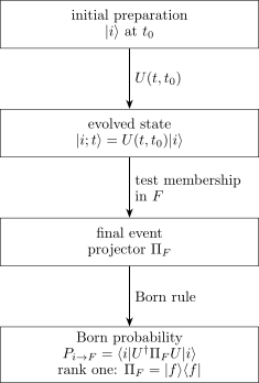
A transition probability combines a preparation, an evolution, and a final event. For a pure initial state and final subspace $F$, the exact probability is $\langle i|U^\dagger\Pi_FU|i\rangle$; a rank-one $\Pi_F$ gives the squared state-to-state amplitude.

Changing any one of these ingredients changes the question. An overlap without time evolution, a dynamical transition, and a conditional post-measurement state are related but distinct objects.

Static state-to-state probability

For normalized pure states $|\psi\rangle$ and $|\phi\rangle$, the static transition amplitude is

$$\mathcal A_{\psi\to\phi} = \langle\phi|\psi\rangle,$$

and

$$P_{\psi\to\phi} = |\langle\phi|\psi\rangle|^2.$$

This is simply the Born probability for the rank-one projector

$$\Pi_\phi = |\phi\rangle\langle\phi|:$$ $$\begin{aligned} \langle\psi|\Pi_\phi|\psi\rangle &= \langle\psi|\phi\rangle \langle\phi|\psi\rangle\\ &= |\langle\phi|\psi\rangle|^2. \end{aligned}$$

Orthogonal states have zero transition probability. Identical rays have unit transition probability.

Normalization and ray invariance

For nonzero unnormalized vectors, the ray-to-ray probability is

$$P_{\psi\to\phi} = \frac{ |\langle\phi|\psi\rangle|^2 }{ \langle\phi|\phi\rangle \langle\psi|\psi\rangle }.$$

For normalized vectors, arbitrary phase changes give

$$|\psi\rangle\mapsto e^{i\alpha}|\psi\rangle, \qquad |\phi\rangle\mapsto e^{i\beta}|\phi\rangle.$$

The amplitude changes by $e^{i(\alpha-\beta)}$, but its modulus does not. Transition probability therefore depends on rays, not vector representatives. The geometry is developed at Projective Hilbert Space.

Transition to a subspace

Often the final event is degenerate or coarse grained. Let $\Pi_F$ project onto a final subspace $F$. Then

$$P_{\psi\to F} = \langle\psi|\Pi_F|\psi\rangle.$$

If $\{|f,\alpha\rangle\}$ is any orthonormal basis of $F$,

$$\Pi_F = \sum_\alpha |f,\alpha\rangle\langle f,\alpha|,$$

so

$$P_{\psi\to F} = \sum_\alpha |\langle f,\alpha|\psi\rangle|^2.$$

The result is basis independent. Orthogonal alternatives within the resolved subspace contribute probabilities because the final measurement distinguishes their projectors or deliberately coarse-grains over mutually exclusive outcomes.

Coherent and exclusive alternatives

The instruction “sum amplitudes, then square” applies when multiple indistinguishable alternatives lead to the same final event. The instruction “sum probabilities” applies to exclusive outcomes whose records are distinguishable or have been decohered.

For example, if one final ray can be reached through amplitudes $\mathcal A_1$ and $\mathcal A_2$, then

$$P = |\mathcal A_1+\mathcal A_2|^2$$

contains the interference term

$$2\operatorname{Re}(\mathcal A_1^*\mathcal A_2).$$

By contrast, transition into an unresolved orthogonal subspace gives

$$P_F = \sum_\alpha |\mathcal A_\alpha|^2$$

with no cross terms between the orthogonal final projectors.

Unitary dynamical transition

Suppose a closed system is prepared in $|i\rangle$ at $t_0$. At time $t$,

$$|i;t\rangle = U(t,t_0)|i\rangle.$$

The amplitude for final state $|f\rangle$ is

$$\mathcal A_{i\to f}(t,t_0) = \langle f|U(t,t_0)|i\rangle,$$

and the transition probability is

$$P_{i\to f}(t,t_0) = |\mathcal A_{i\to f}(t,t_0)|^2.$$

For a final subspace,

$$\begin{aligned} P_{i\to F}(t,t_0) &= \langle i;t|\Pi_F|i;t\rangle\\ &= \langle i|U(t,t_0)^\dagger \Pi_FU(t,t_0)|i\rangle. \end{aligned}$$

The exact construction and composition law for $U$ are at Time-Evolution Operator.

State and effect pictures

The same probability can be calculated by evolving the state forward or the final projector backward. Define

$$\Pi_F(t_0;t) \equiv U(t,t_0)^\dagger\Pi_FU(t,t_0).$$

Then

$$P_{i\to F}(t,t_0) = \langle i|\Pi_F(t_0;t)|i\rangle.$$

This is the Schrödinger–Heisenberg equivalence for the transition question. The physical probability is picture independent; only the bookkeeping of state and measurement operators changes.

Mixed initial states

For a density operator $\rho(t_0)$, unitary evolution gives

$$\rho(t) = U(t,t_0)\rho(t_0)U(t,t_0)^\dagger.$$

The probability of final subspace $F$ is

$$P_{\rho\to F}(t,t_0) = \operatorname{Tr}\!\left[ \Pi_F\rho(t) \right].$$

Equivalently,

$$\begin{aligned} P_{\rho\to F}(t,t_0) &= \operatorname{Tr}\!\left[ \Pi_FU\rho U^\dagger \right]\\ &= \operatorname{Tr}\!\left[ \rho U^\dagger\Pi_FU \right], \end{aligned}$$

where the time arguments on $U$ are suppressed on the second display. For a rank-one final projector,

$$P_{\rho\to f}(t,t_0) = \langle f|\rho(t)|f\rangle.$$

There is generally no single initial ket whose amplitude can replace the trace for a mixed preparation.

Channels and generalized final events

An open-system evolution is represented by a quantum channel $\mathcal E_{t,t_0}$ rather than by $U\rho U^\dagger$ on the system alone. A general final event is represented by a POVM effect $E_F$, with $0\le E_F\le I$. The transition probability is

$$P_{\rho\to F}(t,t_0) = \operatorname{Tr}\!\left[ E_F\,\mathcal E_{t,t_0}(\rho) \right].$$

This formula includes projective closed-system transitions as a special case. In general it cannot be reduced to one squared system amplitude. The channel formalism is introduced at Quantum Channels and Noise.

Composition through an intermediate basis

Let $t_0<t_1<t_2$ and insert a complete orthonormal basis at $t_1$:

$$I = \sum_n|n\rangle\langle n|.$$

The exact amplitude composition law is

$$\begin{aligned} \langle f|U(t_2,t_0)|i\rangle &= \sum_n \langle f|U(t_2,t_1)|n\rangle\\ &\quad\times \langle n|U(t_1,t_0)|i\rangle. \end{aligned}$$

No measurement has been assumed at $t_1$. The intermediate labels are coherent alternatives, so their amplitudes are summed before taking a modulus squared.

What an intermediate measurement changes

Suppose instead that a rank-one projective measurement in the basis $\{|n\rangle\}$ is physically performed at $t_1$, and its outcome is ignored. The probability becomes

$$\begin{aligned} P^{\mathrm{unread}}_{i\to f} &= \sum_n |\langle f|U(t_2,t_1)|n\rangle|^2\\ &\quad\times |\langle n|U(t_1,t_0)|i\rangle|^2. \end{aligned}$$

The interference terms between different $n$ are gone because the measurement has created distinguishable records, even if no one reads them. This is not a mere algebraic insertion of the identity; it is a different physical process.

Sequential measurement and conditioning are treated at Sequential Measurements.

Transition-probability matrices

Choose orthonormal initial and final bases in a finite $d$-dimensional Hilbert space and define

$$T_{fi} \equiv |\langle f|U|i\rangle|^2.$$

Unitarity implies column normalization,

$$\sum_fT_{fi}=1,$$

and row normalization,

$$\sum_iT_{fi}=1.$$

Thus $T$ is doubly stochastic. It records transition probabilities but discards the phases of $U$; many different unitaries can produce the same $T$. Not every doubly stochastic matrix is of this form in dimensions greater than two; those that are are called unistochastic.

Energy eigenstates under a fixed Hamiltonian

For a time-independent Hamiltonian,

$$H|E_n\rangle = E_n|E_n\rangle,$$

and

$$U(t,t_0)|E_n\rangle = e^{-iE_n(t-t_0)/\hbar}|E_n\rangle.$$

Therefore

$$\langle E_m|U(t,t_0)|E_n\rangle = e^{-iE_n(t-t_0)/\hbar}\delta_{mn},$$

so

$$P_{E_n\to E_m}(t,t_0) = \delta_{mn}.$$

Evolution under $H$ alone does not transfer an exact energy eigenstate to a different eigenspace of the same $H$. Transitions among unperturbed energy levels require an additional interaction, a time-dependent Hamiltonian, an open-system process, or a different final measurement basis.

Symmetry selection rules

Suppose a self-adjoint symmetry generator $G$ is conserved by the evolution,

$$[U(t,t_0),G]=0,$$

and the initial and final states satisfy

$$G|i\rangle=g_i|i\rangle, \qquad G|f\rangle=g_f|f\rangle.$$

Then

$$(g_f-g_i) \langle f|U(t,t_0)|i\rangle =0.$$

If $g_f\ne g_i$, the amplitude vanishes. This is the abstract origin of many selection rules. A zero transition can therefore follow from symmetry, not from insufficient elapsed time or a small interaction.

Continuous final sectors

Let generalized final eigenstates obey

$$\langle\lambda,\alpha|\lambda',\alpha'\rangle = \delta_{\alpha\alpha'} \delta(\lambda-\lambda').$$

For a normalizable initial state, the probability density with respect to $d\lambda$ is

$$p(\lambda;t) = \sum_\alpha |\langle\lambda,\alpha|U(t,t_0)|i\rangle|^2.$$

The probability of an interval $\Delta$ is

$$P_{i\to\Delta}(t,t_0) = \int_\Delta p(\lambda;t)\,d\lambda.$$

The generalized amplitude has units determined by the delta-normalization convention, and an exact continuum value ordinarily has zero probability. One must not square a delta function or interpret a continuum amplitude density as a dimensionless probability. See Born Rule for Continuous Spectra.

Survival amplitude and probability

The survival amplitude of an initial pure state is

$$\mathcal S_\psi(t,t_0) = \langle\psi|U(t,t_0)|\psi\rangle.$$

The survival probability is

$$S_\psi(t,t_0) = |\mathcal S_\psi(t,t_0)|^2.$$

An energy eigenstate of a time-independent Hamiltonian has $S_\psi=1$. A superposition of energies can have a time-dependent survival probability because its components acquire relative phases.

Quadratic short-time survival

For $U(\tau)=e^{-iH\tau/\hbar}$ and a state with finite energy variance,

$$\begin{aligned} \mathcal S_\psi(\tau) &= 1- \frac{i\tau}{\hbar}\langle H\rangle\\ &\quad- \frac{\tau^2}{2\hbar^2}\langle H^2\rangle +o(\tau^2). \end{aligned}$$

Taking the squared modulus gives

$$S_\psi(\tau) = 1- \frac{(\Delta H)^2}{\hbar^2}\tau^2 +o(\tau^2).$$

The initial departure is quadratic, not linear. Repeated sufficiently frequent tests can therefore modify survival dynamics, the starting point for Quantum Zeno Dynamics.

Example: spin precession

Let

$$H = \frac{\hbar\Omega}{2}\sigma_z, \qquad |i\rangle=|+x\rangle.$$

Using

$$|\pm x\rangle = \frac{|+z\rangle\pm|-z\rangle}{\sqrt2},$$

the evolved state is

$$|i;t\rangle = \frac{ e^{-i\Omega t/2}|+z\rangle + e^{i\Omega t/2}|-z\rangle }{\sqrt2}.$$

The amplitude for $|-x\rangle$ is

$$\begin{aligned} \langle-x|i;t\rangle &= \frac12\left( e^{-i\Omega t/2}-e^{i\Omega t/2} \right)\\ &= -i\sin\frac{\Omega t}{2}. \end{aligned}$$

Therefore

$$P_{+x\to-x}(t) = \sin^2\frac{\Omega t}{2},$$

while

$$P_{+x\to+x}(t) = \cos^2\frac{\Omega t}{2}.$$

The unitary state evolves continuously. The probabilities refer to a later projective measurement in the $x$ basis; they do not describe hidden random jumps between the two rays.

Forward and reversed transitions

For any unitary $U$,

$$P_{i\to f}[U] = |\langle f|U|i\rangle|^2 = P_{f\to i}[U^\dagger].$$

The reverse process uses the inverse evolution. In general,

$$P_{i\to f}[U] \ne P_{f\to i}[U].$$

Equality under the same forward protocol requires additional structure, such as an applicable time-reversal or reciprocity symmetry. Unitarity alone should not be mistaken for microscopic reciprocity under an unchanged drive.

Probability is not a rate

A finite-time transition probability is dimensionless. A rate has units of inverse time. The instantaneous derivative

$$\frac{d}{dt}P_{i\to f}(t)$$

can vary with time and can even be negative when probability flows back from the chosen final subspace. It is not automatically a constant decay or transition rate.

For isolated discrete states, exact short-time transition probabilities are typically quadratic in time. A nearly constant rate emerges only under additional approximations, often involving weak coupling, a dense continuum, coarse time resolution, and a Markovian window. Those assumptions are the domain of Fermi’s Golden Rule.

Exact probabilities and approximations

The exact formula

$$P_{i\to f}(t,t_0) = |\langle f|U(t,t_0)|i\rangle|^2$$

is simple even when $U$ is hard to calculate. Time-dependent perturbation theory approximates the amplitude when a weak interaction couples known unperturbed states. The canonical first-order construction is First-Order Transition Probability.

Transition Rates separates microscopic rate, finite-time probability, decay width, cross section, lifetime, and detector count rate in spectroscopy.

Measurement update is a separate question

The number $P_{i\to F}$ predicts how often the final event occurs. If the final measurement is actually performed and $F$ is selected, a conditional state update follows. That update is not contained in the probability alone.

For an ideal projective measurement, see Projective Measurement and State Update Rule.

Common mistakes

Calling an amplitude a probability

$\langle f|U|i\rangle$ is generally complex. The probability is its squared modulus.

Omitting evolution between different times

If preparation and final test occur at different times, insert the physical evolution operator or channel. A bare overlap answers a different question.

Summing probabilities for coherent alternatives

When no intermediate record distinguishes alternatives, sum amplitudes before squaring. Summing probabilities discards interference and models a different process.

Summing amplitudes over orthogonal final outcomes

If a final event coarse-grains mutually exclusive orthogonal outcomes, sum their Born probabilities. The projector onto the subspace enforces this rule.

Treating generalized eigenstates as normalized vectors

Continuum labels produce probability densities and interval probabilities. Delta-normalized kets do not define nonzero exact-value probabilities by a naive squared overlap.

Confusing probability with state update

A predicted event probability does not specify the conditional state after the event. Measurement instruments and update rules carry additional data.

Applying unitary formulas to open evolution

For an open system, use a quantum channel and a final effect. A single system amplitude generally does not exist.

Replacing a finite-time probability by a constant rate

A rate requires dynamical and coarse-graining assumptions. Dividing any probability by elapsed time does not automatically produce a meaningful rate.

Summary

For a normalized pure preparation, unitary evolution, and final ray,

$$P_{i\to f}(t,t_0) = |\langle f|U(t,t_0)|i\rangle|^2.$$

For a mixed state, channel, and general final effect,

$$P_{\rho\to F}(t,t_0) = \operatorname{Tr}\!\left[ E_F\mathcal E_{t,t_0}(\rho) \right].$$

Subspace projectors handle degeneracy and coarse graining. Intermediate alternatives add coherently unless a physical measurement or environment creates distinguishable records. Continuum transitions are described by probability densities and intervals. Transition probabilities are exact dimensionless Born predictions; rates and perturbative formulas require additional assumptions.

References

• P. Busch, P. J. Lahti, J.-P. Pellonpää, and K. Ylinen, Quantum Measurement, Springer, 2016, Chapters 3–5.
• C. Cohen-Tannoudji, B. Diu, and F. Laloë, Quantum Mechanics, Vols. I–II, Wiley, 1977.
• P. A. M. Dirac, The Principles of Quantum Mechanics, 4th ed., Oxford University Press, 1958, Chapters II–V.
• J. J. Sakurai and J. Napolitano, Modern Quantum Mechanics, 3rd ed., Cambridge University Press, 2020, Chapters 2 and 5.
• R. Shankar, Principles of Quantum Mechanics, 2nd ed., Springer, 1994, Chapters 4 and 14.
• J. von Neumann, Mathematical Foundations of Quantum Mechanics, Princeton University Press, 1955, Chapters III–V.

Exercises

1. Transition to a degenerate subspace

Let $|1\rangle,|2\rangle,|3\rangle$ be orthonormal and

$$|\psi\rangle = \frac{|1\rangle+2|2\rangle+i|3\rangle}{\sqrt6}.$$

Find the probability that a measurement projects the state into $F=\operatorname{span}\{|1\rangle,|3\rangle\}$.

Solution

The projector is

$$\Pi_F = |1\rangle\langle1|+|3\rangle\langle3|.$$

The two orthogonal probabilities add:

$$\begin{aligned} P_{\psi\to F} &= |\langle1|\psi\rangle|^2 + |\langle3|\psi\rangle|^2\\ &= \frac16+\frac16 = \frac13. \end{aligned}$$

2. Spin-precession transition

For $H=(\hbar\Omega/2)\sigma_z$ and initial state $|+x\rangle$, find the earliest positive time at which a measurement in the $x$ basis returns $|-x\rangle$ with certainty.

Solution

The transition probability is

$$P_{+x\to-x}(t) = \sin^2\frac{\Omega t}{2}.$$

It first equals one when $\Omega t/2=\pi/2$, so

$$t=\frac{\pi}{\Omega}.$$

3. Coherent paths versus an unread measurement

Let a qubit start in $|0\rangle$, evolve by a Hadamard gate $H$, and then by a second $H$ before a final $|0\rangle$ test. Compare the probability with no intermediate measurement to the probability when the computational basis is measured after the first gate and the result is ignored.

Solution

Without an intermediate measurement,

$$H^2=I,$$

so the final state is $|0\rangle$ and

$$P_{0\to0}=1.$$

After the first Hadamard, an unread computational-basis measurement gives $|0\rangle$ or $|1\rangle$ with probability $1/2$. From either state, the second Hadamard gives final $|0\rangle$ probability $1/2$. Hence

$$P^{\mathrm{unread}}_{0\to0} = \frac12\frac12+ \frac12\frac12 = \frac12.$$

The intermediate measurement removes the interference that made the two Hadamards cancel coherently.

4. Doubly stochastic transition matrix

For finite-dimensional unitary $U$, prove that

$$T_{fi}=|\langle f|U|i\rangle|^2$$

has every row and column summing to one.

Solution

Completeness of the final basis and $U^\dagger U=I$ give

$$\begin{aligned} \sum_fT_{fi} &= \sum_f\langle i|U^\dagger|f\rangle \langle f|U|i\rangle\\ &= \langle i|U^\dagger U|i\rangle =1. \end{aligned}$$

Completeness of the initial basis and $UU^\dagger=I$ similarly give

$$\sum_iT_{fi} = \langle f|UU^\dagger|f\rangle =1.$$

5. A symmetry-forbidden transition

Let the self-adjoint generator $G$ commute with $U$, and suppose $G|i\rangle=g_i|i\rangle$ and $G|f\rangle=g_f|f\rangle$ with $g_i\ne g_f$. Prove that the transition probability vanishes.

Solution

Using $GU=UG$,

$$\begin{aligned} g_f\langle f|U|i\rangle &= \langle f|GU|i\rangle\\ &= \langle f|UG|i\rangle\\ &= g_i\langle f|U|i\rangle. \end{aligned}$$

Thus

$$(g_f-g_i)\langle f|U|i\rangle=0.$$

Because $g_f\ne g_i$, the amplitude and hence its squared modulus vanish.

6. Short-time survival law

Assuming finite energy variance, start from

$$\mathcal S(\tau) = 1-\frac{i\tau}{\hbar}\langle H\rangle -\frac{\tau^2}{2\hbar^2}\langle H^2\rangle +o(\tau^2),$$

show that

$$|\mathcal S(\tau)|^2 = 1-\frac{(\Delta H)^2}{\hbar^2}\tau^2 +o(\tau^2).$$

Solution

Write $\mu=\langle H\rangle$ and $m_2=\langle H^2\rangle$, both real. Then

$$\mathcal S^*(\tau) = 1+\frac{i\tau}{\hbar}\mu -\frac{\tau^2}{2\hbar^2}m_2 +o(\tau^2).$$

Multiplication gives

$$\begin{aligned} |\mathcal S(\tau)|^2 &= 1- \frac{m_2-\mu^2}{\hbar^2}\tau^2 +o(\tau^2)\\ &= 1- \frac{(\Delta H)^2}{\hbar^2}\tau^2 +o(\tau^2). \end{aligned}$$

7. A continuous final distribution

For $\lambda\ge0$, suppose the final amplitude density is

$$a(\lambda) = \sqrt{\frac{2}{\Lambda}} e^{-\lambda/\Lambda},$$

and it vanishes for $\lambda<0$. Verify normalization and find the probability of $0\le\lambda\le\Lambda$.

Solution

The probability density is

$$p(\lambda) = \frac{2}{\Lambda}e^{-2\lambda/\Lambda}.$$

It is normalized because

$$\int_0^\infty \frac{2}{\Lambda}e^{-2\lambda/\Lambda}\,d\lambda =1.$$

The requested interval probability is

$$\begin{aligned} P(0\le\lambda\le\Lambda) &= \int_0^\Lambda \frac{2}{\Lambda}e^{-2\lambda/\Lambda}\,d\lambda\\ &= 1-e^{-2}. \end{aligned}$$

The amplitude density has units $[\lambda]^{-1/2}$, while $p(\lambda)$ has units $[\lambda]^{-1}$.

8. Open-system transition under amplitude damping

A qubit begins in $|1\rangle\langle1|$ and undergoes an amplitude-damping channel with parameter $0\le\gamma\le1$ and Kraus operators

$$K_0 = |0\rangle\langle0| + \sqrt{1-\gamma}|1\rangle\langle1|,$$

and

$$K_1 = \sqrt\gamma|0\rangle\langle1|.$$

Find the final probabilities of $|0\rangle$ and $|1\rangle$.

Solution

The evolved state is

$$\begin{aligned} \mathcal E(|1\rangle\langle1|) &= K_0|1\rangle\langle1|K_0^\dagger + K_1|1\rangle\langle1|K_1^\dagger\\ &= (1-\gamma)|1\rangle\langle1| + \gamma|0\rangle\langle0|. \end{aligned}$$

Therefore

$$P_{1\to0}=\gamma, \qquad P_{1\to1}=1-\gamma.$$

The system evolution is nonunitary, so these probabilities are computed from the channel output rather than one system transition amplitude.