Autler–Townes Splitting

Autler–Townes splitting is the appearance of two spectroscopic resonances when a strong coherent field couples two states that would otherwise contribute one probe resonance. In the simplest resonant case, the separation approaches the control-field Rabi frequency:

$$\Delta\omega_{\mathrm{AT}} \simeq \Omega_c.$$

The statement is asymptotic, not definitional. A Hamiltonian may have two dressed eigenvalues before an experiment resolves two peaks, and a narrow transparency dip can appear through interference even when the response poles have not split. A trustworthy interpretation therefore combines:

• the control-dressed eigenvalues and matrix elements;
• a weak-probe open-system response;
• linewidth, Doppler, propagation, and instrument models;
• explicit alternatives such as power broadening and electromagnetically induced transparency.

The effect was introduced in microwave spectroscopy by Autler and Townes in 1955 and is also called resonant dynamic Stark splitting. It now appears in atomic, molecular, solid-state, cavity, circuit, and Rydberg-field spectroscopy.

Canonical Scope

This page owns the weak-probe spectroscopy of a strongly coupled three-state system:

1. the probe–control ladder Hamiltonian and detuning conventions;
2. dressed resonance positions, separation, and probe strengths;
3. the linear probe coherence and absorption profile with decoherence;
4. pole splitting, peak visibility, and instrumental resolvability;
5. distinctions from one-line power broadening and interference-based EIT;
6. effects of control detuning, Doppler shifts, spatial averaging, and multilevel structure;
7. extraction of Rabi frequencies, dipole moments, and electric fields;
8. reproducible fitting and uncertainty checks.

Nearby pages retain distinct responsibilities:

• Dressed States owns the eigenvector transformation, mixing angles, atom–photon manifolds, and Floquet dictionary.
• Optical Bloch Equations owns the driven two-state master equation, saturation, and ordinary power broadening.
• Line Shapes and Broadening owns natural, lifetime, collision, Doppler, inhomogeneous, and instrumental width conventions.
• AC Stark Shift owns far-detuned branch shifts and optical potentials.
• Cavity QED owns input–output spectra, cavity loss, cooperativity, and vacuum normal-mode splitting.

The next page, Electromagnetically Induced Transparency, owns dark states, destructive pathway interference, transparency-window dispersion, slow light, and memory connections. The present page derives only enough of the shared weak-probe response to distinguish EIT from a resolved Autler–Townes doublet.

Probe–Control Ladder

States and fields

Use a ladder with energies

$$E_g<E_e<E_r$$

and transition frequencies

$$\omega_{eg} = \frac{E_e-E_g}{\hbar}, \qquad \omega_{re} = \frac{E_r-E_e}{\hbar}.$$

A weak probe of angular frequency $\omega_p$ couples $|g\rangle\leftrightarrow|e\rangle$ with Rabi-frequency coefficient $\Omega_p$. A stronger control of angular frequency $\omega_c$ couples $|e\rangle\leftrightarrow|r\rangle$ with coefficient $\Omega_c$.

Use atom-minus-field detunings

$$\Delta_p = \omega_{eg}-\omega_p, \qquad \Delta_c = \omega_{re}-\omega_c,$$

and the ladder two-photon detuning

$$\delta = \Delta_p+\Delta_c.$$

Thus red detuning is positive. Frequencies, detunings, couplings, and decay rates are angular quantities unless a factor of $2\pi$ is displayed.

Rotating-frame Hamiltonian

Choose phases so both Rabi coefficients are real and nonnegative. In the ordered basis

$$\left( |g\rangle, |e\rangle, |r\rangle \right),$$

the rotating-wave Hamiltonian is

$$\frac{H}{\hbar} = \begin{pmatrix} 0 & \Omega_p/2 & 0 \\ \Omega_p/2 & \Delta_p & \Omega_c/2 \\ 0 & \Omega_c/2 & \delta \end{pmatrix}.$$

This model assumes:

1. the two fields address only the displayed transitions;
2. both rotating-wave approximations are controlled;
3. the probe is weak enough for linear response;
4. a single velocity, position, polarization pathway, and control amplitude are considered before ensemble averaging;
5. dissipation can be represented by Markovian coherence rates.

An open chain has enough state-phase freedom to make both couplings real. A closed loop driven on all three transitions can retain an observable loop phase and requires a different analysis.

Control-Dressed Resonances

Strong-coupling subspace

In the weak-probe limit, set $\Omega_p\to0$ while retaining the probe frequency as the scanned reference. The coupled $|e\rangle,|r\rangle$ subblock is

$$\frac{H_{er}}{\hbar} = \begin{pmatrix} \Delta_p & \Omega_c/2 \\ \Omega_c/2 & \Delta_p+\Delta_c \end{pmatrix}.$$

Its eigenvalues relative to the uncoupled $|g\rangle$ quasienergy are

$$\lambda_\pm = \Delta_p + \frac{\Delta_c}{2} \pm \frac{\Omega_{R,c}}{2},$$

where

$$\Omega_{R,c} = \sqrt{ \Delta_c^2+\Omega_c^2 }.$$

The weak probe becomes resonant when one dressed branch is degenerate with $|g\rangle$:

$$\lambda_\pm=0.$$

Therefore the ideal resonance detunings are

$$\Delta_p^{(\pm)} = \frac{ -\Delta_c \pm \Omega_{R,c} }{ 2 }.$$

Their separation and midpoint are

$$\Delta_p^{(+)} - \Delta_p^{(-)} = \Omega_{R,c},$$

and

$$\frac{ \Delta_p^{(+)} + \Delta_p^{(-)} }{ 2 } = - \frac{\Delta_c}{2}.$$

For resonant control,

$$\Delta_c=0,$$

the ideal pair lies at

$$\Delta_p = \pm\frac{\Omega_c}{2},$$

so its separation is $\Omega_c$.

Probe matrix elements

Define the control mixing angle by

$$\cos\theta_c = \frac{\Delta_c}{\Omega_{R,c}}, \qquad \sin\theta_c = \frac{\Omega_c}{\Omega_{R,c}}.$$

After removing the common energy and ordering the control-coupled basis as $(|r\rangle,|e\rangle)$, one convenient choice is

$$\begin{aligned} |+\rangle_c &= \cos\frac{\theta_c}{2}|r\rangle + \sin\frac{\theta_c}{2}|e\rangle, \\ |-\rangle_c &= - \sin\frac{\theta_c}{2}|r\rangle + \cos\frac{\theta_c}{2}|e\rangle. \end{aligned}$$

Because the probe couples $|g\rangle$ to the $|e\rangle$ component, the ideal squared matrix-element weights associated with the algebraic roots above are

$$\begin{aligned} W_+ &= \frac12 \left( 1+\frac{\Delta_c}{\Omega_{R,c}} \right), \\ W_- &= \frac12 \left( 1-\frac{\Delta_c}{\Omega_{R,c}} \right). \end{aligned}$$

Here $W_+$ accompanies the root

$$\Delta_p^{(+)} = \frac{ -\Delta_c+\Omega_{R,c} }{2},$$

not the upper quasienergy label $|+\rangle_c$. This explicit convention avoids a common branch-label swap.

At control resonance, $W_+=W_-=1/2$. For large positive $\Delta_c$, the near-zero probe root has $W_+\to1$, while the far root becomes weak. Peak heights need not equal these weights because decay, populations, interference, optical depth, and the detection channel also enter.

Far-detuned limit

If

$$\Delta_c>0, \qquad \Delta_c\gg\Omega_c,$$

then

$$\Omega_{R,c} \simeq \Delta_c + \frac{\Omega_c^2}{2\Delta_c}.$$

The bright near-zero root becomes

$$\Delta_p^{(+)} \simeq \frac{\Omega_c^2}{4\Delta_c},$$

whereas the weak remote root lies near

$$\Delta_p^{(-)} \simeq - \Delta_c - \frac{\Omega_c^2}{4\Delta_c}.$$

The near-root displacement is the AC Stark shift of the probe transition in this detuning convention. Autler–Townes splitting and perturbative light shifts are therefore the resonant and far-detuned limits of the same avoided crossing, but different language is useful in the two regimes.

Weak-Probe Response

Coherence decay rates

Let:

• $\gamma_{ge}$ be the decay rate of the probe coherence $\rho_{ge}$;
• $\gamma_{gr}$ be the decay rate of the two-photon coherence $\rho_{gr}$.

These are homogeneous angular-frequency HWHM parameters in the coherence equations. They can include population decay and pure dephasing. For example, in a simple model,

$$\gamma_{ge} = \frac{\Gamma_g+\Gamma_e}{2} + \gamma_{ge}^*,$$

with an analogous expression for $\gamma_{gr}$. Usually $\Gamma_g=0$, but the formula makes the convention explicit.

Linearized optical Bloch equations

Assume the probe is weak enough that

$$\rho_{gg} \simeq 1, \qquad \rho_{ee}, \rho_{rr} = O(\Omega_p^2).$$

To first order in $\Omega_p$, the slowly varying coherences obey

$$\begin{aligned} \dot\rho_{ge} &= - \left( \gamma_{ge}-i\Delta_p \right) \rho_{ge} \\ &\quad + i\frac{\Omega_p}{2} + i\frac{\Omega_c}{2}\rho_{gr}, \\ \dot\rho_{gr} &= - \left( \gamma_{gr}-i\delta \right) \rho_{gr} \\ &\quad + i\frac{\Omega_c}{2}\rho_{ge}. \end{aligned}$$

The control creates a second coherence path. Solving the steady equations gives

$$\frac{\rho_{ge}}{\Omega_p} = \frac{i}{2} \frac{ \gamma_{gr}-i\delta }{ \left( \gamma_{ge}-i\Delta_p \right) \left( \gamma_{gr}-i\delta \right) + \Omega_c^2/4 }.$$

With this phase convention, define the normalized absorption proxy

$$\mathcal A(\Delta_p) \equiv \operatorname{Im} \left( \frac{\rho_{ge}}{\Omega_p} \right).$$

The physical susceptibility has a positive prefactor containing number density and the probe dipole matrix element. When the control is absent,

$$\mathcal A_0(\Delta_p) = \frac{ \gamma_{ge} }{ 2 \left( \Delta_p^2+\gamma_{ge}^2 \right) },$$

which is one homogeneous Lorentzian.

Resonant-control profile

Set $\Delta_c=0$, so $\delta=\Delta_p$, and define

$$a = \gamma_{ge}\gamma_{gr} + \frac{\Omega_c^2}{4}, \qquad b = \gamma_{ge}+\gamma_{gr}.$$

The absorption proxy becomes

$$\mathcal A(\Delta_p) = \frac{ \gamma_{ge}\Delta_p^2 + \gamma_{gr}a }{ 2 \left[ \left( a-\Delta_p^2 \right)^2 + b^2\Delta_p^2 \right] }.$$

At line center,

$$\mathcal A(0) = \frac{ \gamma_{gr} }{ 2 \left( \gamma_{ge}\gamma_{gr} + \Omega_c^2/4 \right) }.$$

Relative to the no-control line-center absorption,

$$\frac{ \mathcal A(0) }{ \mathcal A_0(0) } = \frac{ \gamma_{ge}\gamma_{gr} }{ \gamma_{ge}\gamma_{gr} + \Omega_c^2/4 }.$$

This formula is central to the EIT distinction. If $\gamma_{gr}$ is very small, substantial line-center transparency can occur for a control that is too weak to create split response poles.

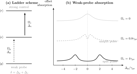
Left: a weak probe addresses $|g\rangle\leftrightarrow|e\rangle$ while a stronger control couples $|e\rangle\leftrightarrow|r\rangle$. Right: normalized, vertically offset weak-probe absorption from the resonant three-level model with $\gamma_{gr}=0.08\gamma_{ge}$. The middle trace has a central interference dip although its poles are not yet split; the strong control produces a resolved Autler–Townes doublet.

Poles, Peaks, and Resolvability

Complex response poles

For resonant control, the denominator has complex poles

$$\begin{aligned} \Delta_{p,\mathrm{pole}}^{(\pm)} &= \pm \frac12 \sqrt{ \Omega_c^2 - \left( \gamma_{ge}-\gamma_{gr} \right)^2 } \\ &\quad - i \frac{ \gamma_{ge}+\gamma_{gr} }{ 2 }. \end{aligned}$$

The poles acquire distinct real parts when

$$\Omega_c > \left| \gamma_{ge}-\gamma_{gr} \right|.$$

This is a useful pole-splitting criterion for the stated linear, resonant, homogeneous model. It is not a universal experimental resolution criterion.

In the strong-control limit,

$$\Omega_c \gg \gamma_{ge}, \gamma_{gr},$$

the pole separation approaches $\Omega_c$, and each isolated component has an approximate pole HWHM

$$\gamma_{\mathrm{pole}} \simeq \frac{ \gamma_{ge}+\gamma_{gr} }{ 2 }.$$

The actual maximum of $\mathcal A$ can differ from the real part of a pole when the components overlap or their residues interfere. Near the crossover, fitting two independent Lorentzians and calling their fitted distance “the Rabi frequency” can be biased.

What counts as resolved

Two peaks are experimentally resolved only relative to a stated forward model and noise level. Relevant scales include:

• homogeneous component widths;
• Doppler and other inhomogeneous distributions;
• spatial variation of $\Omega_c$;
• probe-laser and control-laser noise;
• instrument response and scan calibration;
• optical depth and propagation;
• background, sampling interval, and signal-to-noise ratio.

A conservative strong-splitting statement is

$$\Omega_c \gg \gamma_{ge}, \gamma_{gr}, \sigma_{\mathrm{inh}}, \delta\omega_{\mathrm{inst}},$$

where the last two symbols summarize inhomogeneous and instrumental scales. The symbol $\gg$ deliberately avoids pretending that one Rayleigh-like number applies to every line shape and estimator.

Peak separation is not always the eigenvalue gap

In the lossless model,

$$\Delta\omega_{\mathrm{gap}} = \Omega_{R,c}.$$

In data, one may instead quote:

1. the difference between local maxima;
2. the difference between fitted component centers;
3. the real-part separation of response poles;
4. the Hamiltonian dressed-state gap.

These quantities agree in the well-resolved weak-probe limit. They need not agree near threshold. A publication or calibration should say which one was used.

Difference from Power Broadening

Ordinary two-level power broadening concerns one transition driven and observed in the same saturated response. In the convention of Optical Bloch Equations, its FWHM is

$$w_{\mathrm{pow}} = 2\Gamma_2 \sqrt{ 1+s_0 }.$$

The center remains one resonance in the ideal model, while the response flattens and widens with intensity.

Autler–Townes spectroscopy instead uses a strong control to couple one transition and a weak probe to interrogate a connected transition. In the well-resolved regime:

• power broadening: one wider component;
• Autler–Townes splitting: two dressed components.

Real data can contain both. The control broadens and decoheres the dressed components, the probe can saturate if it is not weak, and optical pumping can redistribute population. The correct comparison is therefore between forward models, not between the words “broad” and “split.”

Useful diagnostics are:

• the squared splitting should follow

  $$\left( \Delta\omega_{\mathrm{AT}} \right)^2 \simeq \Delta_c^2+\Omega_c^2;$$

• at resonant control, $\Omega_c\propto E_c\propto\sqrt{I_c}$;

• detuning should move the midpoint by $-\Delta_c/2$ and exchange the component strengths;

• a one-line saturation model should fail systematically once two components are resolved.

Difference from EIT

Two mechanisms for a central dip

Autler–Townes splitting and electromagnetically induced transparency can both produce reduced absorption near the center of a probe line.

Autler–Townes mechanism. A strong control separates two absorptive response poles. The low absorption between them is primarily the valley between resolved resonances.

EIT mechanism. Coherent excitation pathways interfere destructively at two-photon resonance. A narrow transparency window can be carved inside an otherwise unsplit broad resonance.

For the resonant model above, deep line-center suppression requires

$$\frac{ \Omega_c^2 }{ 4\gamma_{ge}\gamma_{gr} } \gg 1.$$

Pole splitting requires

$$\Omega_c > \left| \gamma_{ge}-\gamma_{gr} \right|.$$

When

$$\gamma_{gr} \ll \gamma_{ge},$$

there can be a broad interval in which the first condition is satisfied but the second is not. A narrow, high-contrast dip in that interval is interference dominated rather than a resolved Autler–Townes doublet.

Crossover, not a universal border

The two limiting pictures are valuable, but not every spectrum belongs unambiguously to one category. Multilevel degeneracy, unequal decay paths, Doppler averaging, optical depth, and finite resolution move the crossover. In an intermediate regime, both dressed-pole separation and interference shape the same response.

A responsible analysis can:

1. fit the full complex susceptibility derived from the physical level scheme;
2. compare constrained EIT-like and ATS-like reduced models;
3. use an information criterion or predictive validation rather than raw residual size alone;
4. report when the evidence is inconclusive.

The Akaike-information approach introduced by Anisimov, Dowling, and Sanders and tested in cold cesium by Giner and collaborators is one such model-comparison strategy. It does not remove the need to model the actual level structure and experimental convolution.

Configuration matters

For a Λ system, the two-photon coherence connects two long-lived lower states and can have

$$\gamma_{gr} \ll \gamma_{ge}.$$

That hierarchy strongly favors a narrow EIT window.

For a ladder, the two-photon coherence includes the upper-state lifetime and may decay more rapidly. For a V system, the relevant upper-state coherence, shared ground state, and control-induced population changes alter the response. It is unsafe to transfer one ATS/EIT threshold among Λ, ladder, and V schemes without rederiving the coherence equations.

Detuned and Asymmetric Doublets

Control detuning does three things:

1. increases the ideal branch separation from $\Omega_c$ to $\Omega_{R,c}$;
2. moves the pair midpoint to $-\Delta_c/2$ in the present convention;
3. makes the probe matrix-element weights unequal.

The two roots satisfy the invariants

$$\Delta_p^{(+)} + \Delta_p^{(-)} = -\Delta_c,$$

and

$$\Delta_p^{(+)} \Delta_p^{(-)} = - \frac{\Omega_c^2}{4}.$$

These relations are useful calibration checks. A common-mode scan offset changes the measured sum but not the separation. An incorrect detuning sign reverses the expected motion of the midpoint and strength exchange.

Asymmetry can also arise from:

• unequal dressed-state matrix elements;
• unequal decay and branching;
• nearby spectator states;
• polarization-dependent Clebsch–Gordan coefficients;
• control-induced optical pumping;
• Doppler selection;
• dispersive detection or interference with a background field.

Therefore asymmetric peaks do not, by themselves, prove control detuning.

What the Detector Measures

Absorption and transmission

In a dilute, uniform, weak-probe medium,

$$\alpha(\omega_p) \propto \operatorname{Im}\chi(\omega_p) \propto \mathcal A(\Delta_p).$$

For propagation length $L$,

$$T(\omega_p) = \exp \left[ - \alpha(\omega_p)L \right].$$

At small optical depth,

$$1-T \simeq \alpha L.$$

At larger optical depth, a Lorentzian absorption coefficient does not produce a Lorentzian transmission curve. Fitting transmission directly with a sum of Lorentzians can distort widths and areas.

Dispersion and phase

The real part of the susceptibility changes the probe phase and group delay. A central absorption minimum can coexist with steep dispersion. That dispersion is central to EIT applications, but an Autler–Townes doublet also has dispersive structure. A measured phase slope alone does not establish a dark state.

Fluorescence and population readout

Fluorescence often measures an excited-state population times branching, collection efficiency, and detector response:

$$R_{\mathrm{det}} = \eta \sum_j \Gamma_{j\to\mathrm{det}} \rho_{jj}.$$

It is not generally proportional to $\operatorname{Im}\chi$. State ionization, loss, shelving, and quantum-jump counts define still other observables. A spectrum can show peaks in one channel and dips in another without contradicting the same dressed dynamics.

Convolution and sampling

A practical forward model may be written schematically as

$$y_i = B(\omega_i) + \left( R_{\mathrm{inst}}\ast S_{\mathrm{phys}} \right) (\omega_i) + \epsilon_i,$$

where the convolution means

$$\begin{aligned} \left( R_{\mathrm{inst}}\ast S_{\mathrm{phys}} \right) (\omega_i) &= \int R_{\mathrm{inst}} \left( \omega_i-\omega \right) \\ &\quad\times S_{\mathrm{phys}}(\omega) \,d\omega. \end{aligned}$$

Here $B$ is a baseline, $R_{\mathrm{inst}}$ is the instrument response, $S_{\mathrm{phys}}$ is the predicted absorption, transmission, or count signal, and $\epsilon_i$ is noise. The scan-axis calibration and point spacing belong to the model, not merely to plot formatting.

Motion and Spatial Averaging

Doppler detunings

For an atom of velocity $\mathbf v$, the observed field frequencies are Doppler shifted. With the atom-minus-field convention,

$$\Delta_p(\mathbf v) = \Delta_p + \mathbf k_p\mathbin{\cdot}\mathbf v,$$

and

$$\Delta_c(\mathbf v) = \Delta_c + \mathbf k_c\mathbin{\cdot}\mathbf v.$$

For the ladder,

$$\delta(\mathbf v) = \delta + \left( \mathbf k_p+\mathbf k_c \right) \mathbin{\cdot}\mathbf v.$$

The vector signs include beam direction. Counter-propagating beams can reduce the two-photon Doppler width when their wave-vector magnitudes are similar; unequal wavelengths leave a residual.

The ensemble response is

$$\overline{\chi}(\omega_p) = \int f(\mathbf v) \chi \left[ \Delta_p(\mathbf v), \Delta_c(\mathbf v) \right] d^3v.$$

One should average the complex susceptibility before converting it to transmission. Averaging fitted peak centers afterward is not generally equivalent.

Control-beam profile

For electric-dipole coupling,

$$\Omega_c(\mathbf r) = \frac{ \left| \mathbf d_{re} \mathbin{\cdot} \boldsymbol\epsilon_c \right| E_c(\mathbf r) }{ \hbar }.$$

A Gaussian control beam produces a distribution of local splittings. The observed signal is weighted by probe intensity, density, detection efficiency, and sometimes optical pumping:

$$S_{\mathrm{obs}} \propto \int d^3r\, n(\mathbf r) I_p(\mathbf r) S_{\mathrm{loc}} \left[ \Omega_c(\mathbf r) \right].$$

Using peak control intensity when the experiment measures a spatial average biases an inferred dipole moment or electric field.

Transit and pulse effects

Steady-state formulas require interaction times long compared with the relevant coherence-settling times. Short pulses add Fourier width and can create transient Rabi ringing. Moving particles can sample a time-dependent control envelope even under continuous illumination. A pulsed Autler–Townes experiment should solve the time-dependent density matrix and model the detector gate.

Multilevel and Polarization Effects

Real atoms and molecules rarely provide one isolated ladder. The control may couple several Zeeman, hyperfine, rotational, or vibrational states:

$$\Omega_{c,m} = \frac{ E_c }{ \hbar } \left| \langle r,m_r| \mathbf d\mathbin{\cdot}\boldsymbol\epsilon_c |e,m_e\rangle \right|.$$

Different angular factors produce several splittings. Unresolved components can broaden, skew, or multiply the observed lines.

A controlled calculation should:

1. choose a quantization axis from the applied fields;
2. enumerate probe and control selection rules;
3. include all states within several coupling strengths or linewidths;
4. propagate optical pumping among magnetic sublevels;
5. average over polarization impurities and field inhomogeneity;
6. test whether one effective dipole matrix element is identifiable.

For precision electrometry, ambiguity among magnetic-sublevel transition moments can dominate the calibration. Isolating one angular-momentum pathway is often more valuable than merely increasing signal.

Extracting Couplings and Fields

Rabi frequency from a splitting

In the resolved weak-probe regime, fit the generalized relation

$$S^2 = \Delta_c^2+\Omega_c^2,$$

where $S$ is the dressed gap or a justified estimator of it. At nominal resonance,

$$\Omega_c \simeq S.$$

Near the resolution threshold, use the full response rather than replacing $S$ by the distance between raw local maxima.

Transition dipole moment

For a linearly polarized peak electric field $E_0$,

$$\Omega_c = \frac{ \left| \mathbf d_{re} \mathbin{\cdot}\boldsymbol\epsilon_c \right| E_0 }{ \hbar }.$$

If the measured splitting in cycles per second is

$$\nu_{\mathrm{AT}} = \frac{\Omega_c}{2\pi},$$

then

$$\left| \mathbf d_{re} \mathbin{\cdot}\boldsymbol\epsilon_c \right| = \frac{ h\nu_{\mathrm{AT}} }{ E_0 }.$$

The field must be the local field at the sample, not merely one inferred from laser power before windows, focusing, standing waves, or cavity enhancement.

Electric-field sensing

If the transition dipole is known, the same equation measures a resonant electric field:

$$E_0 = \frac{ \hbar\Omega_c }{ \left| \mathbf d_{re} \mathbin{\cdot}\boldsymbol\epsilon_c \right| }.$$

Rydberg transitions have large dipole moments, making their Autler–Townes splitting useful for radio-frequency and microwave electrometry. “Atom based” does not mean uncertainty free. A traceable measurement still requires:

• correct state and angular factor;
• local-field and polarization characterization;
• frequency-axis traceability;
• a validated splitting estimator;
• treatment of cell perturbations, standing waves, and field gradients;
• uncertainty propagation for theoretical matrix elements.

Square-root intensity test

For a plane wave,

$$I_c = \frac12 c\epsilon_0E_0^2.$$

Therefore

$$\Omega_c \propto \sqrt{I_c},$$

and, at fixed detuning,

$$S^2 = \Delta_c^2 + \beta I_c.$$

A linear fit of $S^2$ against calibrated local intensity separates a detuning intercept from the coupling slope. Deviations can reveal saturation of the readout, changing beam size, multilevel crossings, or an incorrect peak estimator.

Applications

Double-resonance spectroscopy

The control dresses a transition that may be difficult to observe directly, while a convenient probe reads out the splitting. This enables assignments, matrix-element measurements, and tests of level mixing in atoms and molecules.

Rydberg electrometry

An optical ladder prepares and reads a Rydberg state while a microwave or radio-frequency field couples neighboring Rydberg levels. The optical spectrum converts a high-frequency electric field into a measurable Autler–Townes separation. Rydberg Electrometry develops the resulting inverse problem, including unresolved-field methods, polarization, vapor-cell transfer, bandwidth, and traceability.

Solid-state and artificial atoms

Quantum dots, color centers, superconducting circuits, and other few-level systems can show the same pump–probe structure. Their dephasing, spectral diffusion, selection rules, and readout channels differ from dilute atomic gases, so the shared square-root Hamiltonian does not imply a shared line-shape model.

Quantized control fields

If the control is a quantized cavity mode, its coupling in an excitation manifold scales as

$$\Omega_c \longrightarrow 2g\sqrt N.$$

Vacuum-induced or photon-number-resolved splittings can then reveal the quantized mode. Cavity transmission additionally depends on $\kappa$, input–output interference, and photon statistics; it should be analyzed with the cavity-QED forward model rather than the classical-control formula alone.

A Reliable Analysis Workflow

1. Draw the actual level graph. Mark every probe, control, decay, and repumping connection.
2. Declare conventions. Give basis order, detuning signs, Rabi-frequency factors, field amplitude, and linewidth units.
3. Verify the weak-probe limit. Check linear scaling of signal with probe power and absence of probe-induced shifts or broadening.
4. Fit the no-control spectrum first. Infer baseline, homogeneous and inhomogeneous widths, scan calibration, and instrument response.
5. Calibrate control detuning independently. Do not infer it only from an already asymmetric doublet.
6. Use the full complex response near crossover. Reserve two independent Lorentzians for a demonstrably separated pair.
7. Average the physical model. Include velocity, position, polarization, and multilevel distributions before applying transmission or detector nonlinearities.
8. Compare alternatives. Test one-line broadening, interference-dip, and split-pole models where each is plausible.
9. Check scaling. Verify $S^2=\Delta_c^2+\Omega_c^2$ and $\Omega_c\propto\sqrt{I_c}$ over a controlled range.
10. Propagate calibration uncertainty. Include dipole, field, frequency, beam profile, model selection, and estimator bias.

Common Mistakes

Calling any central dip Autler–Townes splitting

A narrow interference minimum can appear without split poles. Check the control scale against both $\sqrt{\gamma_{ge}\gamma_{gr}}$ and $|\gamma_{ge}-\gamma_{gr}|$.

Calling any two fitted Lorentzians two dressed states

Flexible component fits can split an asymmetric or non-Lorentzian line even when the physical response has one unresolved structure. Compare constrained forward models.

Equating eigenvalue separation with visible peak distance

Loss and interference move maxima away from pole real parts near crossover. State the estimator and use the full response when the pair overlaps.

Ignoring the probe

A probe that is not weak changes populations, coherences, and linewidths. It can dress the system itself and invalidate the linear susceptibility.

Mixing hertz and radians per second

If a measured separation is quoted in hertz, use

$$\Omega_c = 2\pi\nu_{\mathrm{AT}}.$$

Using $\hbar\nu_{\mathrm{AT}}$ instead of $h\nu_{\mathrm{AT}}$ in a field calibration loses a factor of $2\pi$.

Using nominal power as the local field

Window loss, focusing, standing waves, cavity enhancement, polarization, and spatial averaging separate source power from the field sampled by the particles.

Treating component heights as bare-state probabilities

Peak heights also depend on linewidths, populations, propagation, detector response, and interference. Even integrated areas equal simple dressed weights only under stated limiting assumptions.

Forgetting control detuning

A detuned control changes the separation, midpoint, and strength ratio. Fitting the separation as $\Omega_c$ overestimates the coupling when $\Delta_c\ne0$.

Averaging spectra after taking transmission

For an inhomogeneous medium, average the susceptibility or local propagation model in the physically correct order. Exponentiation and averaging do not generally commute.

Importing a Λ threshold into a ladder or V system

The long-lived coherence and decay pathways differ among configurations. Derive the relevant linear equations for the actual state graph.

Claiming traceability from atomic structure alone

Atomic frequencies and matrix elements are valuable references, but the measurement chain still includes state preparation, local fields, polarization, geometry, model discrepancy, and readout calibration.

Key Results

The ideal probe resonances are

$$\Delta_p^{(\pm)} = \frac{ -\Delta_c \pm \sqrt{ \Delta_c^2+\Omega_c^2 } }{ 2 }.$$

Their ideal separation is

$$\Delta\omega_{\mathrm{AT}} = \sqrt{ \Delta_c^2+\Omega_c^2 },$$

and at control resonance it approaches $\Omega_c$.

For a compact statement of the weak-probe coherence, define

$$\begin{aligned} D(\Delta_p) &= \left( \gamma_{ge}-i\Delta_p \right) \\ &\quad\times \left[ \gamma_{gr} - i(\Delta_p+\Delta_c) \right] + \frac{\Omega_c^2}{4}. \end{aligned}$$

Then

$$\frac{\rho_{ge}}{\Omega_p} = \frac{i}{2} \frac{ \gamma_{gr}-i(\Delta_p+\Delta_c) }{ D(\Delta_p) }.$$

For resonant control, response poles split in real frequency when

$$\Omega_c > \left| \gamma_{ge}-\gamma_{gr} \right|.$$

Deep interference transparency instead requires the weaker scale

$$\Omega_c^2 \gg 4\gamma_{ge}\gamma_{gr}.$$

The separation of those two conditions is why a central dip does not, by itself, identify Autler–Townes splitting.

Further Connections

• Rabi Oscillations measures the same coherent coupling through time-domain population exchange.
• Dynamic Polarizability places the strong-control response in the broader frequency-dependent susceptibility framework.
• Electromagnetically Induced Transparency develops the unsplit dark-state regime, dispersive delay, and spin-coherence storage.
• Rydberg Atoms Basics explains the large transition moments used in microwave electrometry.
• Rydberg Electrometry carries the splitting into a complete local- or external-field estimate.
• Precision Spectroscopy develops calibrated scans, line-center inference, systematic shifts, and uncertainty budgets.
• Resonant Driving gives the general driven-transition approximation hierarchy.

References

1. S. H. Autler and C. H. Townes, “Stark effect in rapidly varying fields,” Physical Review 100, 703–722 (1955).
2. C. Cohen-Tannoudji, J. Dupont-Roc, and G. Grynberg, Atom–Photon Interactions: Basic Processes and Applications (Wiley, 1992).
3. B. W. Shore, The Theory of Coherent Atomic Excitation (Wiley, 1990).
4. T. Y. Abi-Salloum, “Electromagnetically induced transparency and Autler–Townes splitting: Two similar but distinct phenomena in two categories of three-level atomic systems,” Physical Review A 81, 053836 (2010).
5. P. M. Anisimov, J. P. Dowling, and B. C. Sanders, “Objectively discerning Autler–Townes splitting from electromagnetically induced transparency,” Physical Review Letters 107, 163604 (2011); arXiv:1102.0546.
6. L. Giner et al., “Experimental investigation of the transition between Autler–Townes splitting and electromagnetically-induced- transparency models,” Physical Review A 87, 013823 (2013); arXiv:1206.5921.
7. M. Fleischhauer, A. Imamoglu, and J. P. Marangos, “Electromagnetically induced transparency: Optics in coherent media,” Reviews of Modern Physics 77, 633–673 (2005).
8. B. D. Gerardot et al., “Dressed excitonic states and quantum interference in a three-level quantum dot ladder system,” New Journal of Physics 11, 013028 (2009); arXiv:0803.0432.
9. A. Sanli et al., “Measurement of the $\mathrm{Na}_2$ transition dipole moments using optical–optical double resonance and Autler–Townes spectroscopy,” Journal of Chemical Physics 147, 204301 (2017).
10. N. Schlossberger et al., “Calibration of Autler–Townes based electrometry in Rydberg states of alkali atoms,” 2024 Conference on Precision Electromagnetic Measurements (2024); NIST record.

Exercises

1. Derive the dressed probe resonances

Diagonalize

$$\frac{H_{er}}{\hbar} = \begin{pmatrix} \Delta_p & \Omega_c/2 \\ \Omega_c/2 & \Delta_p+\Delta_c \end{pmatrix}.$$

Find the probe detunings at which either eigenvalue crosses zero. Verify the sum and product of those detunings.

Solution

The trace and difference of the diagonal entries are

$$\operatorname{Tr} \left( \frac{H_{er}}{\hbar} \right) = 2\Delta_p+\Delta_c,$$

and

$$\left( \Delta_p+\Delta_c \right) - \Delta_p = \Delta_c.$$

Hence

$$\lambda_\pm = \Delta_p + \frac{\Delta_c}{2} \pm \frac12 \sqrt{ \Delta_c^2+\Omega_c^2 }.$$

Setting $\lambda_\pm=0$ gives the unordered pair

$$\Delta_p^{(\pm)} = \frac{ -\Delta_c \pm \sqrt{ \Delta_c^2+\Omega_c^2 } }{2}.$$

Their sum is

$$\Delta_p^{(+)} + \Delta_p^{(-)} = -\Delta_c,$$

and their product is

$$\begin{aligned} \Delta_p^{(+)} \Delta_p^{(-)} &= \frac{ \Delta_c^2 - \left( \Delta_c^2+\Omega_c^2 \right) }{4} \\ &= - \frac{\Omega_c^2}{4}. \end{aligned}$$

Both checks are independent of the branch-label convention.

2. Convert a Rydberg splitting into electric field

A resonant microwave field produces a measured splitting

$$\nu_{\mathrm{AT}} = 18.0\pm0.2\ \mathrm{MHz}.$$

The relevant projected dipole moment is

$$d = (900\pm18)\,ea_0.$$

Find the peak electric field and its standard uncertainty, neglecting correlations and all other systematics. Use

$$e = 1.602176634\times10^{-19}\ \mathrm C,$$

and

$$a_0 = 5.291772109\times10^{-11}\ \mathrm m.$$

Solution

Because the measured splitting is in cycles per second,

$$E_0 = \frac{ h\nu_{\mathrm{AT}} }{ d }.$$

The dipole is

$$\begin{aligned} d &= 900 \left( 1.602176634\times10^{-19} \right) \\ &\quad\times \left( 5.291772109\times10^{-11} \right) \ \mathrm{C\,m} \\ &\simeq 7.63\times10^{-27}\ \mathrm{C\,m}. \end{aligned}$$

Using

$$h = 6.62607015\times10^{-34}\ \mathrm{J\,s},$$

the numerator is

$$h\nu_{\mathrm{AT}} \simeq 1.193\times10^{-26}\ \mathrm{J}.$$

Therefore

$$\begin{aligned} E_0 &\simeq \frac{ 1.193\times10^{-26} }{ 7.63\times10^{-27} } \\ &\simeq 1.56\ \mathrm{V\,m^{-1}}. \end{aligned}$$

For independent uncertainties,

$$\left( \frac{u_E}{E_0} \right)^2 = \left( \frac{0.2}{18.0} \right)^2 + \left( \frac{18}{900} \right)^2.$$

Thus

$$\frac{u_E}{E_0} \simeq 0.0229, \qquad u_E \simeq 0.036\ \mathrm{V\,m^{-1}}.$$

The result under the restricted assumptions is

$$E_0 = (1.56\pm0.04)\ \mathrm{V\,m^{-1}}.$$

A real uncertainty budget must add state purity, polarization, local-field, line-shape, scan-axis, and matrix-element model uncertainties.

3. Derive the weak-probe coherence

Starting from

$$\begin{aligned} 0 &= - \left( \gamma_{ge}-i\Delta_p \right) \rho_{ge} + i\frac{\Omega_p}{2} + i\frac{\Omega_c}{2}\rho_{gr}, \\ 0 &= - \left( \gamma_{gr}-i\delta \right) \rho_{gr} + i\frac{\Omega_c}{2}\rho_{ge}, \end{aligned}$$

solve for $\rho_{ge}/\Omega_p$. Check the result when $\Omega_c=0$.

Solution

The second equation gives

$$\rho_{gr} = \frac{ i\Omega_c\rho_{ge}/2 }{ \gamma_{gr}-i\delta }.$$

Insert this into the first equation:

$$\begin{aligned} i\frac{\Omega_p}{2} &= \left[ \gamma_{ge}-i\Delta_p \right. \\ &\qquad\left. + \frac{ \Omega_c^2 }{ 4 \left( \gamma_{gr}-i\delta \right) } \right] \rho_{ge}. \end{aligned}$$

Multiplying numerator and denominator by $\gamma_{gr}-i\delta$ yields

$$\frac{\rho_{ge}}{\Omega_p} = \frac{i}{2} \frac{ \gamma_{gr}-i\delta }{ \left( \gamma_{ge}-i\Delta_p \right) \left( \gamma_{gr}-i\delta \right) + \Omega_c^2/4 }.$$

When $\Omega_c=0$, the factor $\gamma_{gr}-i\delta$ cancels:

$$\frac{\rho_{ge}}{\Omega_p} = \frac{i}{ 2 \left( \gamma_{ge}-i\Delta_p \right) }.$$

Its imaginary part is

$$\frac{ \gamma_{ge} }{ 2 \left( \Delta_p^2+\gamma_{ge}^2 \right) },$$

the expected positive Lorentzian absorption proxy.

4. Classify split poles and transparency

Suppose

$$\frac{\gamma_{ge}}{2\pi} = 6.0\ \mathrm{MHz}, \qquad \frac{\gamma_{gr}}{2\pi} = 0.20\ \mathrm{MHz}.$$

1. Find the resonant-control pole-splitting threshold.
2. Find the scale $2\sqrt{\gamma_{ge}\gamma_{gr}}$ at which line-center suppression becomes appreciable.
3. Classify controls with $\Omega_c/(2\pi)=3.0\ \mathrm{MHz}$ and $12.0\ \mathrm{MHz}$.
4. For the stronger control, calculate the real pole separation and pole HWHM in megahertz.

Solution

All rates contain the same factor of $2\pi$, so the comparisons can be made using their values in megahertz.

The split-pole threshold is

$$\frac{ \Omega_{c,\mathrm{th}} }{ 2\pi } = 6.0-0.20 = 5.8\ \mathrm{MHz}.$$

The interference-suppression scale is

$$\begin{aligned} \frac{ 2\sqrt{ \gamma_{ge}\gamma_{gr} } }{ 2\pi } &= 2\sqrt{ (6.0)(0.20) } \ \mathrm{MHz} \\ &\simeq 2.19\ \mathrm{MHz}. \end{aligned}$$

The $3.0\ \mathrm{MHz}$ control exceeds the transparency scale but is below the split-pole threshold. It can produce an EIT-like central dip, but not two poles with distinct real parts in this model.

The $12.0\ \mathrm{MHz}$ control exceeds the threshold and lies in the Autler–Townes regime. Its real pole separation is

$$\begin{aligned} \frac{S_{\mathrm{pole}}}{2\pi} &= \sqrt{ 12.0^2 - \left( 6.0-0.20 \right)^2 } \ \mathrm{MHz} \\ &\simeq 10.5\ \mathrm{MHz}. \end{aligned}$$

The pole HWHM is

$$\begin{aligned} \frac{\gamma_{\mathrm{pole}}}{2\pi} &= \frac{6.0+0.20}{2} \ \mathrm{MHz} \\ &= 3.10\ \mathrm{MHz}. \end{aligned}$$

Whether the two maxima are cleanly resolved still depends on the numerator, inhomogeneous width, and instrument response.

5. Detuned doublet positions and strengths

Take

$$\frac{\Delta_c}{2\pi} = 10.0\ \mathrm{MHz}, \qquad \frac{\Omega_c}{2\pi} = 6.0\ \mathrm{MHz}.$$

Neglect decay. Find the generalized splitting, both probe resonance detunings, the midpoint, and the ideal squared matrix-element weights $W_+$ and $W_-$.

Solution

The generalized splitting is

$$\begin{aligned} \frac{\Omega_{R,c}}{2\pi} &= \sqrt{ 10.0^2+6.0^2 } \ \mathrm{MHz} \\ &\simeq 11.66\ \mathrm{MHz}. \end{aligned}$$

The roots are

$$\begin{aligned} \frac{ \Delta_p^{(+)} }{ 2\pi } &= \frac{-10.0+11.66}{2} \ \mathrm{MHz} \\ &\simeq 0.83\ \mathrm{MHz}, \end{aligned}$$

and

$$\begin{aligned} \frac{ \Delta_p^{(-)} }{ 2\pi } &= \frac{-10.0-11.66}{2} \ \mathrm{MHz} \\ &\simeq -10.83\ \mathrm{MHz}. \end{aligned}$$

Their midpoint is $-5.00\ \mathrm{MHz}$. The weights are

$$\begin{aligned} W_+ &= \frac12 \left( 1+\frac{10.0}{11.66} \right) \simeq 0.929, \\ W_- &= \frac12 \left( 1-\frac{10.0}{11.66} \right) \simeq 0.071. \end{aligned}$$

The near-zero resonance is bright and the far resonance is weak. A large eigenvalue separation therefore need not yield two peaks of comparable visibility.

6. Deep transparency without split poles

Let

$$\gamma_{ge} = 5.0, \qquad \gamma_{gr} = 0.050,$$

in common angular-frequency units.

1. For $\Omega_c=1.0$, calculate the ratio $\mathcal A(0)/\mathcal A_0(0)$.
2. Find the minimum $\Omega_c$ that suppresses line-center absorption by $90\%$.
3. Compare that value with the pole-splitting threshold.

Solution

The center ratio is

$$R = \frac{ \gamma_{ge}\gamma_{gr} }{ \gamma_{ge}\gamma_{gr} + \Omega_c^2/4 }.$$

Here

$$\gamma_{ge}\gamma_{gr} = (5.0)(0.050) = 0.25,$$

and $\Omega_c^2/4=0.25$, so

$$R = \frac{0.25}{0.50} = 0.50.$$

For $90\%$ suppression, require $R\le0.10$:

$$\frac{ \gamma_{ge}\gamma_{gr} }{ \gamma_{ge}\gamma_{gr} + \Omega_c^2/4 } \le 0.10.$$

This gives

$$\Omega_c^2 \ge 36\gamma_{ge}\gamma_{gr},$$

so

$$\Omega_c \ge 6\sqrt{0.25} = 3.0.$$

The split-pole threshold is

$$\left| \gamma_{ge}-\gamma_{gr} \right| = 4.95.$$

Thus a $90\%$ central transparency can occur at $\Omega_c=3.0$ even though the poles are not split. The dip is interference dominated in this regime.

7. Two-photon Doppler width

A ladder uses a $780\ \mathrm{nm}$ probe and a $480\ \mathrm{nm}$ control. For a one-dimensional velocity RMS of

$$\sigma_v = 0.20\ \mathrm{m\,s^{-1}},$$

estimate the RMS two-photon Doppler width in hertz for:

1. co-propagating beams;
2. counter-propagating beams.

Treat both quoted wavelengths as vacuum wavelengths.

Solution

In cycles per second, the two-photon Doppler coefficient is the signed sum of inverse wavelengths:

$$\sigma_\nu = \left| \frac{s_p}{\lambda_p} + \frac{s_c}{\lambda_c} \right| \sigma_v,$$

where $s_p,s_c=\pm1$ encode beam directions.

For co-propagating beams,

$$\begin{aligned} \sigma_\nu^{\mathrm{co}} &= \left( \frac1{780\times10^{-9}} + \frac1{480\times10^{-9}} \right) \\ &\quad\times (0.20) \\ &\simeq 6.73\times10^5\ \mathrm{Hz} \\ &= 0.673\ \mathrm{MHz}. \end{aligned}$$

For counter-propagating beams,

$$\begin{aligned} \sigma_\nu^{\mathrm{counter}} &= \left| \frac1{780\times10^{-9}} - \frac1{480\times10^{-9}} \right| \\ &\quad\times (0.20) \\ &\simeq 1.60\times10^5\ \mathrm{Hz} \\ &= 0.160\ \mathrm{MHz}. \end{aligned}$$

Counter-propagation reduces the two-photon Doppler width by about a factor of $4.2$, but it does not cancel it because the wavelengths differ.

8. Audit positions and areas

Two well-separated probe features are fitted at

$$\begin{aligned} \frac{\Delta_{p,1}}{2\pi} &= -4.0\ \mathrm{MHz}, \\ \frac{\Delta_{p,2}}{2\pi} &= +6.0\ \mathrm{MHz}. \end{aligned}$$

Assume the ideal lossless ladder model.

1. Infer $\Delta_c/(2\pi)$ and $\Omega_c/(2\pi)$.
2. Predict the ideal squared matrix-element weight ratio for the $+6.0\ \mathrm{MHz}$ and $-4.0\ \mathrm{MHz}$ roots.
3. An experiment instead reports an integrated-area ratio $4:1$. Explain what can and cannot be concluded.

Solution

The root sum gives

$$\frac{ \Delta_{p,1}+\Delta_{p,2} }{ 2\pi } = 2.0\ \mathrm{MHz} = - \frac{\Delta_c}{2\pi}.$$

Therefore

$$\frac{\Delta_c}{2\pi} = -2.0\ \mathrm{MHz}.$$

The separation is

$$\frac{\Omega_{R,c}}{2\pi} = 10.0\ \mathrm{MHz}.$$

Hence

$$\begin{aligned} \frac{\Omega_c}{2\pi} &= \sqrt{ 10.0^2-(-2.0)^2 } \ \mathrm{MHz} \\ &\simeq 9.80\ \mathrm{MHz}. \end{aligned}$$

The positive root has

$$W_+ = \frac12 \left( 1+\frac{-2.0}{10.0} \right) = 0.40,$$

while the negative root has

$$W_- = 0.60.$$

The ideal squared matrix-element ratio is therefore

$$W_+:W_- = 2:3,$$

not $4:1$.

The positions remain consistent with one effective coupling and detuning, but the area discrepancy shows that the simplest identification of integrated area with dressed $|e\rangle$ weight is invalid. Possible causes include unequal linewidths, dressed populations, branching, optical depth, interference, polarization-dependent pathways, unresolved sublevels, background, or detector response. The area mismatch does not erase the position-based coupling inference, but it requires an expanded forward model before claiming quantitative state composition.