Rydberg Electrometry

A Rydberg electrometer infers an electric-field property from the large dipole response of a highly excited atom. In the most common vapor-cell implementation, two optical fields create Rydberg electromagnetically induced transparency (EIT), a radio-frequency field couples the addressed Rydberg state to a neighboring state, and probe transmission supplies the data. The familiar Autler–Townes formula can then convert a resolved spectral splitting into a local field amplitude.

That one-line conversion is the middle of a measurement, not its beginning or end. A complete result must say which field component and amplitude convention are estimated, how a laser scan maps onto an atomic energy interval, how the glass cell changes the incident field, which atoms and positions contribute, and how the recorded photons determine an uncertainty. These distinctions are especially important when the splitting is unresolved, the field is detuned, or the desired measurand is the field outside the cell.

This page is the canonical home for the end-to-end Rydberg-electrometry inverse problem: operating regimes, field-to-spectrum forward models, likelihoods, sensitivity and bandwidth, polarization reconstruction, cell-transfer corrections, and evidence standards. Rydberg Atoms Basics owns the high-$n$ spectrum, scaling laws, lifetimes, polarizabilities, and transition dipoles. Electromagnetically Induced Transparency owns dark states and optical propagation, while Autler–Townes Splitting owns the general dressed-state line-shape derivation. Sensing Case Studies retains the historical account of the 2012 vapor-cell demonstration and the subsequent evidence record.

State the Measurement Contract

An electric field is a vector-valued function of position and time. A useful measurement therefore begins with a contract such as

$$\mathcal S_{\mathrm R} = (\theta,\mathcal A,\mathcal C, \mathcal M,\mathcal T,\mathcal E).$$

Here

• $\theta$ is the estimand, such as a local peak amplitude, polarization, carrier detuning, modulation quadrature, or external-field parameter;
• $\mathcal A$ specifies the atomic species, resolved sublevels, temperature, density, and Rydberg preparation;
• $\mathcal C$ contains the optical and radio-frequency controls, scan axis, timing, and local oscillator;
• $\mathcal M$ is the photon-count, voltage, camera, or fluorescence likelihood;
• $\mathcal T$ maps the field outside the apparatus to the field sampled by the atoms; and
• $\mathcal E$ is the estimator, calibration chain, and uncertainty model.

For a nearly monochromatic field, write the real field as

$$\mathbf E(\mathbf r,t) = \operatorname{Re} \left[ \mathbf E_0(\mathbf r) e^{-i\omega t} \right].$$

$\mathbf E_0$ is a peak complex phasor. For a linearly polarized sinusoid, $E_{\mathrm{rms}}=E_0/\sqrt 2$. Autler–Townes Rabi frequencies below use the peak convention. A result quoted in $\mathrm{V\,m^{-1}}$ without saying peak, RMS, or spectral-amplitude convention is incomplete.

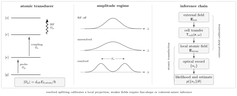
The usual four-level transducer, three amplitude regimes, and the inference chain from an external field to optical data. Atomic structure calibrates the local projected field; an external-field claim additionally requires the cell transfer function and spatial weighting.

Four-Level RF-to-Optical Transducer

States, fields, and detunings

Use a ladder $|g\rangle\leftrightarrow|e\rangle\leftrightarrow|r\rangle$ with probe and coupling Rabi coefficients $\Omega_p$ and $\Omega_c$. A field near angular frequency $\omega_\mu$ couples $|r\rangle$ to a second Rydberg state $|s\rangle$ with coefficient $\Omega_\mu$. Define atom-minus-field detunings

$$\begin{aligned} \Delta_p &= \omega_{eg}-\omega_p,\\ \Delta_c &= \omega_{re}-\omega_c,\\ \Delta_\mu &= \omega_{sr}-\omega_\mu, \end{aligned}$$

and cumulative detunings

$$\delta_2 = \Delta_p+\Delta_c, \qquad \delta_3 = \Delta_p+\Delta_c+\Delta_\mu.$$

Angular frequencies are used unless $2\pi$ is written explicitly. In a rotating-wave frame, one convenient Hamiltonian is

$$\frac{H}{\hbar} = \begin{pmatrix} 0 & \Omega_p^*/2 & 0 & 0\\ \Omega_p/2 & \Delta_p & \Omega_c^*/2 & 0\\ 0 & \Omega_c/2 & \delta_2 & \Omega_\mu^*/2\\ 0 & 0 & \Omega_\mu/2 & \delta_3 \end{pmatrix}.$$

The model is useful only after specifying the states hidden inside each label. Hyperfine and Zeeman sublevels, unwanted polarization components, nearby Rydberg manifolds, and off-resonant couplings can turn one four-state diagram into many interfering pathways.

The projected RF coupling

For peak phasor $\mathbf E_0$ and a selected transition,

$$\Omega_\mu = -\frac{ \langle s|\mathbf d|r\rangle \mathbin{\cdot} \mathbf E_0 }{\hbar}.$$

Its magnitude is

$$|\Omega_\mu| = \frac{d_{\mathrm{eff}}E_0}{\hbar}, \qquad d_{\mathrm{eff}} = \left| \langle s|\mathbf d|r\rangle \mathbin{\cdot} \widehat{\boldsymbol\epsilon} \right|.$$

The sign and complex phase matter in a closed-loop or coherent-mixing experiment, even though an isolated splitting depends only on $|\Omega_\mu|$. The rotating-wave approximation also requires the counter-rotating and neighboring-transition corrections to remain small on the required uncertainty scale.

Weak-probe optical response

In the weak-probe limit, $\rho_{gg}\simeq1$ and the steady optical coherence can be written as a continued fraction. With coherence half-widths $\gamma_{ge}$, $\gamma_{gr}$, and $\gamma_{gs}$,

$$\frac{2\rho_{ge}}{\Omega_p^*} = \frac{i}{ \gamma_{ge}-i\Delta_p + \dfrac{|\Omega_c|^2/4}{ \gamma_{gr}-i\delta_2 + \dfrac{|\Omega_\mu|^2/4}{ \gamma_{gs}-i\delta_3 } } }.$$

This expression displays the nested transduction: the RF field changes a Rydberg coherence, the coupling field maps that change onto the optical coherence, and propagation maps the coherence onto transmitted light. It is not a universal vapor-cell fit function. Saturation, optical pumping, additional levels, velocity changes during transit, and propagation through appreciable optical depth require optical Bloch or master-equation modeling.

For a dilute homogeneous slice, the probe susceptibility is proportional to $\rho_{ge}/\Omega_p^*$ and the intensity transmission has the form

$$T_p(\Delta_p) = \exp\!\left[ -k_p L\operatorname{Im}\chi(\Delta_p) \right].$$

If spectral bin $j$ records a photon count $n_j$, a basic detector model is

$$n_j \sim \operatorname{Poisson} \left[ \mu_j(\theta,\boldsymbol\lambda) \right],$$

where $\boldsymbol\lambda$ collects laser power, detunings, linewidths, background, gain, and other nuisance parameters. Fitting peak positions is one possible estimator; fitting this physical likelihood is more reliable near the resolution boundary.

Resolved Autler–Townes Electrometry

Resonant and detuned dressed gaps

Ignore the weak optical probe momentarily and diagonalize the RF-coupled Rydberg pair. Relative to $|r\rangle$, its rotating-frame block can be written

$$\frac{H_{rs}}{\hbar} = \begin{pmatrix} 0 & \Omega_\mu^*/2\\ \Omega_\mu/2 & \Delta_\mu \end{pmatrix}.$$

The dressed shifts are

$$\lambda_\pm = \frac{\Delta_\mu}{2} \pm \frac12 \sqrt{ \Delta_\mu^2+|\Omega_\mu|^2 },$$

so the eigenvalue gap is

$$S_\omega = \sqrt{ \Delta_\mu^2+|\Omega_\mu|^2 }.$$

On resonance, $S_\omega=|\Omega_\mu|$. If a justified spectral estimator returns the corresponding splitting $S_\nu=S_\omega/(2\pi)$ in hertz, then

$$E_{0,\mathrm{atom}} = \frac{hS_\nu}{d_{\mathrm{eff}}}.$$

This direct conversion applies to the local, projected, peak field when the RF is resonant and the observed peak separation is a valid estimator of the dressed gap. Off resonance,

$$E_{0,\mathrm{atom}} = \frac{\hbar}{d_{\mathrm{eff}}} \sqrt{S_\omega^2-\Delta_\mu^2}.$$

Near the resolution threshold, raw local maxima need not coincide with the real parts of the response poles. The full line shape should then determine $\Omega_\mu$ and $\Delta_\mu$ jointly.

The scan-axis correction

The atomic gap and the separation on a plotted laser-frequency axis are not always equal. Let a moving atom have signed axial wave vectors $k_p$ and $k_c$. Its optical detunings are

$$\Delta_p(v) = \Delta_p+k_pv, \qquad \Delta_c(v) = \Delta_c+k_cv.$$

When the coupling laser is scanned while a resonant probe selects atoms near $v=0$, the coupling-axis separation directly gives

$$\Delta\nu_c = \frac{|\Omega_\mu|}{2\pi}$$

in the ideal resonant limit. If instead the probe is scanned and the coupling frequency is held fixed, the strongly absorbing velocity class approximately satisfies $\Delta_p(v)=0$. For counter-propagating beams this gives

$$\delta_2 \simeq -\frac{k_c}{k_p}\Delta_p,$$

and therefore

$$\Delta\nu_p \simeq \frac{\nu_p}{\nu_c} \frac{|\Omega_\mu|}{2\pi} = \frac{\lambda_c}{\lambda_p} \frac{|\Omega_\mu|}{2\pi}.$$

Thus a probe-axis splitting must be divided by $\nu_p/\nu_c=\lambda_c/\lambda_p$ before applying the atomic conversion. This result follows from the stated scan and propagation conventions; a memorized wavelength factor can be inverted by changing either one. Finite linewidth, optical pumping, temperature, and multilevel structure can also modify the simple selected-velocity argument, so precision work should fit the velocity-averaged response.

Below the Resolved-Splitting Regime

Line-shape estimation

A field does not become undetectable merely because two peaks cannot be resolved. It can change the EIT depth, width, curvature, or phase. For independent Poisson spectral bins, the classical Fisher information for a field parameter $E$ is

$$F_E = \sum_j \frac{1}{\mu_j(E)} \left( \frac{\partial\mu_j(E)}{\partial E} \right)^2.$$

With nuisance parameters $\boldsymbol\lambda$, the relevant bound comes from the inverse of the full Fisher matrix,

$$\operatorname{Var}(\widehat E) \geq \left[F^{-1}\right]_{EE},$$

not from $1/F_E$ while pretending that laser detuning and contrast are known. The best probe detuning is usually where the expected signal changes steeply and reproducibly, not necessarily at line center. Modulation and balanced or homodyne optical readout can move the estimate away from low-frequency laser noise, but their duty cycle and reference noise belong in the comparison.

If the observable is even in an unknown field, its small-field response may begin as

$$y(E) = y(0)+aE^2+O(E^4).$$

Then $\partial_Ey=0$ at $E=0$: the sign or phase is absent, and the local Fisher information can vanish even with a visibly perturbed spectrum at larger fields. A known bias or coherent local oscillator restores a linear term.

Atomic homodyne and heterodyne mixing

Let a strong local oscillator and a weak signal address the same effective Rydberg transition:

$$\begin{aligned} E_{\mathrm{LO}}(t) &= E_L\cos(\omega_Lt),\\ E_{\mathrm s}(t) &= E_s\cos(\omega_st+\phi). \end{aligned}$$

For $E_s\ll E_L$ and $\omega_s-\omega_L=\omega_{\mathrm{IF}}$ within the atomic and detector bandwidth, the slowly varying envelope is

$$E_{\mathrm{env}}(t) \simeq E_L + E_s\cos(\omega_{\mathrm{IF}}t+\phi).$$

Linearizing an optical observable $y=f(E_{\mathrm{env}})$ gives

$$y(t) \simeq f(E_L) + f'(E_L)E_s \cos(\omega_{\mathrm{IF}}t+\phi).$$

The atoms now down-convert the signal to an intermediate-frequency optical beat note. Its amplitude estimates a signal quadrature and its phase is defined relative to the local oscillator. This extends detection below the resolved Autler–Townes regime and enables coherent reception. The result is not reference-free: local-oscillator amplitude, phase noise, spatial overlap, and detuning are resources and nuisance parameters.

Resonant, Off-Resonant, and Static Fields

Rydberg electrometry spans several physical responses. They should not be collapsed into one calibration formula.

Regime	Dominant observable	Leading field dependence	Information lost without a reference
resonant RF, resolved	Autler–Townes gap	$S_\nu\propto E_0$	absolute carrier phase
resonant RF, unresolved	EIT line shape or mixer beat	model dependent; linear with a coherent bias	phase or sign in an intensity-only measurement
far-detuned RF	differential AC Stark shift	$\Delta\nu\propto E_0^2$	sign and generally carrier phase
static or quasistatic	differential DC Stark shift	$\Delta\nu\propto E_{\mathrm{dc}}^2$ absent a bias	field sign

For a nondegenerate state with scalar static polarizability $\alpha_i(0)$,

$$\Delta U_i^{(\mathrm{dc})} = -\frac12\alpha_i(0)E_{\mathrm{dc}}^2.$$

The measured transition shift is set by the differential polarizability,

$$\Delta\nu_{sr}^{(\mathrm{dc})} = -\frac{ \alpha_s(0)-\alpha_r(0) }{2h} E_{\mathrm{dc}}^2.$$

For a far-off-resonant sinusoid with peak amplitude $E_0$, the cycle average introduces another factor of $1/2$:

$$\Delta U_i^{(\mathrm{ac})} = -\frac14 \alpha_i(\omega)E_0^2.$$

Tensor polarizability, near-degenerate mixing, and strong fields require a Stark-map or Floquet calculation rather than these scalar formulas. The canonical derivations are on Stark Effect in Atoms and Dynamic Polarizability.

A known static bias $E_b$ can linearize a small perturbation $e$:

$$(E_b+e)^2 = E_b^2+2E_be+e^2.$$

It also imports bias calibration and drift. In glass alkali-vapor cells, surface charge can screen low-frequency external fields or create inhomogeneous offsets, so the field at the atoms must be measured or modeled rather than inferred from electrode voltage alone.

Polarization and Vector Reconstruction

Choose a quantization axis and decompose the RF phasor into spherical components,

$$E_q = \mathbf e_q^* \mathbin{\cdot} \mathbf E_0, \qquad q\in\{-1,0,+1\}.$$

For one angular-momentum pathway,

$$\Omega_{m m'}^{(q)} = -\frac{E_q}{\hbar} \langle F'm'|d_q|Fm\rangle,$$

with

$$\langle F'm'|d_q|Fm\rangle = (-1)^{F'-m'} \begin{pmatrix} F'&1&F\\ -m'&q&m \end{pmatrix} \langle F'\|d\|F\rangle.$$

Selection rules therefore make the spectrum a polarization-dependent sum of pathways, not a direct meter of $|\mathbf E|$. Optical pumping changes their weights. Some populated states may be uncoupled and leave an unsplit central feature; others have different dipole moments and broaden or resolve the doublet.

A vector measurement needs enough independent settings to identify the desired phasor parameters. Schematically,

$$\mathbf y = \mathbf f \left( \mathbf E_0, \mathbf B_0, \boldsymbol\epsilon_p, \boldsymbol\epsilon_c, \boldsymbol\lambda \right).$$

Rotating a known quantization axis, changing optical polarizations, resolving Zeeman components, or using multiple transitions can provide independent constraints. The Jacobian with respect to the estimated field components must have full rank after nuisance parameters are included. Measuring three peak separations is not automatically a three-dimensional vector measurement if the same unknown polarization impurity affects all three.

Thermal Motion and Spatial Transfer

Velocity averaging

For velocity distribution $f(v)$, the susceptibility of a dilute thermal ensemble begins with

$$\overline\chi(\Delta_p,\Delta_c) = \int_{-\infty}^{\infty} f(v) \chi \left[ \Delta_p+k_pv, \Delta_c+k_cv \right] \,dv.$$

Counter-propagating probe and coupling beams reduce the residual two-photon Doppler wave vector $k_p+k_c$, but unequal wavelengths prevent perfect cancellation in the common two-photon ladder. Beam angle, transit time, collisions, laser linewidth, and velocity-changing processes further modify the response. Three-photon ladders can be arranged with a smaller net wave vector, trading additional lasers and levels for narrower Doppler response.

The field inside a vapor cell

At carrier frequency $\omega$, write the local field as

$$\mathbf E_{\mathrm{atom}}(\mathbf r,\omega) = \mathsf T_{\mathrm{cell}}(\mathbf r,\omega) \mathbf E_{\mathrm{external}}(\omega).$$

$\mathsf T_{\mathrm{cell}}$ can include dielectric boundary conditions, standing waves, nearby conductors, electrodes, supports, resonators, and polarization rotation. At low frequency it can include charge transport and screening. It is generally a complex, position-dependent tensor rather than a single scalar correction.

The detected spectrum is weighted by probe and coupling intensities and by atomic trajectories. A schematic forward model is

$$\mu_j = \mathcal D_j \left\{ \int d^3r\,dv\, W(\mathbf r,v) \mathcal P \left[ \chi_j (\mathbf E_{\mathrm{atom}},v,\mathbf r) \right] \right\},$$

where $\mathcal P$ denotes optical propagation and $\mathcal D_j$ the detector response. Because splitting, absorption, propagation, and detector averaging are nonlinear, one generally cannot replace the inhomogeneous field by its spatial mean. A field gradient may appear as broadening, unequal peaks, or a multicomponent line shape.

This distinction separates two legitimate measurands:

1. Atomic local field: a weighted field experienced by atoms in the illuminated cell volume.
2. External or incident field: a parameter before the cell, inferred only through a validated electromagnetic and spatial-transfer model.

A subwavelength optical spot can localize the readout more finely than the RF wavelength, but spatial resolution is set by the full weighting kernel, including beam waist, depth of field, atomic motion, camera pixels, and inverse regularization. It is not simply the cell size.

Sensitivity, Bandwidth, and Dynamic Range

A comparison-ready sensitivity

For total averaging time $\tau$ in a stationary white-noise regime, define

$$\sigma_E(\tau) \simeq \frac{\eta_E}{\sqrt\tau},$$

where $\eta_E$ has units $\mathrm{V\,m^{-1}\,Hz^{-1/2}}$. The reported value should identify:

• peak or RMS field;
• local or external field;
• carrier frequency, detuning, and polarization;
• modulation or analysis frequency and resolution bandwidth;
• active volume and spatial weighting;
• optical powers, atomic density, and readout protocol;
• whether dead time and initialization are included; and
• the averaging interval over which $1/\sqrt\tau$ behavior was verified.

For a resolved resonant splitting,

$$\sigma_E = \frac{h}{d_{\mathrm{eff}}} \sigma_{S_\nu},$$

before scan-axis, detuning, and transfer uncertainties. This relation converts a splitting-estimator uncertainty; it does not predict that uncertainty. Photon shot noise, laser amplitude and frequency noise, atomic projection or number fluctuations, thermal radiation, detector noise, and model mismatch all enter through the data likelihood.

Three different bandwidths

The word bandwidth has at least three meanings here.

1. Carrier coverage is the set of RF frequencies addressable by available Rydberg transitions or by Stark, Zeeman, or dressing-based tuning. Broad coverage across configurations is not simultaneous broadband reception.
2. Instantaneous modulation bandwidth is the highest envelope or phase variation faithfully followed at one carrier setting. It depends on optical pumping, Rabi frequencies, coherence, transit replacement, and detector electronics.
3. Measurement bandwidth or resolution bandwidth is the noise-equivalent bandwidth used to turn fluctuations into a spectral sensitivity.

For a first-order response with time constant $\tau_R$,

$$H(\omega_m) = \frac{H(0)}{1+i\omega_m\tau_R}, \qquad f_{3\mathrm{dB}} = \frac{1}{2\pi\tau_R}.$$

In a thermal vapor, the transit estimate

$$\tau_{\mathrm{tr}} \sim \frac{w}{v_\perp}$$

can be comparable to or shorter than internal relaxation times. Smaller beams can increase response speed but reduce atom number and interaction length, so bandwidth and sensitivity are jointly engineered.

Lower and upper field limits

At low amplitude, an Autler–Townes estimator fails when the line shape no longer identifies two branches. Line-shape, modulation, or mixer estimators can continue below that point. At high amplitude, the selected pair is no longer isolated: nearby Rydberg levels, multiple RF photons, spatially varying splittings, counter-rotating terms, ionization, and detector scan range can limit the model. A trustworthy dynamic range is the interval over which linearity, identifiability, and coverage have all been validated.

Traceability and Uncertainty

The resonant local-field chain is attractive because $h$ is exact in the SI and a transition dipole can be calculated from atomic structure:

$$S_\nu \longrightarrow |\Omega_\mu| \longrightarrow E_{0,\mathrm{atom}}.$$

It is better described as atom-referenced than as automatically self-calibrating. The transition identity, polarization projection, scan-axis scale, RF detuning, and line-shape estimator must still be established. To claim an external field, append

$$E_{0,\mathrm{atom}} \longrightarrow \mathsf T_{\mathrm{cell}}^{-1} \longrightarrow E_{0,\mathrm{external}}.$$

For an approximately scalar transfer magnitude $T$ and independent small uncertainties, a useful first budget is

$$\left( \frac{u(E_{\mathrm{external}})}{E_{\mathrm{external}}} \right)^2 \simeq \left(\frac{u(S_\nu)}{S_\nu}\right)^2 + \left(\frac{u(D)}{D}\right)^2 + \left(\frac{u(d_{\mathrm{eff}})}{d_{\mathrm{eff}}}\right)^2 + \left(\frac{u(T)}{T}\right)^2 +u_{\mathrm{model}}^2.$$

$D$ denotes the applicable scan-axis factor. Correlations require covariance terms, and line-shape model discrepancy is often not well represented by a single Gaussian contribution. A robust analysis varies beam position and power, reverses or rotates polarizations, changes scan direction, fits alternative plausible models, maps the cell electromagnetically, and reports which corrections were measured rather than assumed.

Precision and accuracy answer different questions. Repeated spectra can give a small $\sigma_E$ while an incorrect cell transfer, pathway dipole, or frequency scale biases every result. Conversely, a traceable calibration does not guarantee high sensitivity or communications-ready bandwidth.

Worked Calibration Example

Suppose a coupling-laser scan resolves a resonant splitting

$$S_\nu = 1.000\ \mathrm{MHz}$$

for an isolated pathway with

$$d_{\mathrm{eff}} = 1000\,e a_0 = 8.4784\times10^{-27}\ \mathrm{C\,m}.$$

The local peak field is

$$\begin{aligned} E_{0,\mathrm{atom}} &= \frac{hS_\nu}{d_{\mathrm{eff}}}\\ &= 7.815\times10^{-2}\ \mathrm{V\,m^{-1}}\\ &= 0.7815\ \mathrm{mV\,cm^{-1}}. \end{aligned}$$

For a linearly polarized sinusoid,

$$E_{\mathrm{rms,atom}} = 5.526\times10^{-2}\ \mathrm{V\,m^{-1}}.$$

If the same atomic gap were read by scanning a $780\ \mathrm{nm}$ probe while a counter-propagating $480\ \mathrm{nm}$ coupling laser remained fixed, the ideal probe-axis separation would instead be

$$\Delta\nu_p = \frac{480}{780} (1.000\ \mathrm{MHz}) \simeq 0.615\ \mathrm{MHz}.$$

Applying $h\Delta\nu_p/d_{\mathrm{eff}}$ directly would underestimate the field. Finally, if a validated scalar cell model gives $T=0.80$, the inferred external peak field is $E_{0,\mathrm{external}}=0.0977\ \mathrm{V\,m^{-1}}$. The local atomic result does not require that last correction; the external result does.

Choosing an Operating Mode

Goal	Useful mode	Main calibration object	Dominant failure mode
absolute local RF amplitude	resonant resolved splitting	$d_{\mathrm{eff}}$, detuning, scan axis	multilevel or inhomogeneous peaks
very weak coherent signal	RF homodyne or heterodyne	LO amplitude, phase, transfer gain	reference noise and drift
polarization	resolved sublevels and varied axes	angular pathways and optical polarization	rank-deficient reconstruction
off-resonant carrier	AC Stark or dressed-state model	dynamic polarizability or Floquet spectrum	quadratic ambiguity and nearby levels
low-frequency or DC field	DC Stark shift with bias or electrodes	differential polarizability and screening	wall charge and field inhomogeneity
field image	camera or scanned optical volume	spatial kernel and cell map	interpreting pixel size as resolution
communication waveform	locked optical readout and mixer	transfer function and linear range	confusing data rate with carrier coverage

No mode is universally best. Resolved splitting provides a transparent frequency-to-field conversion but has a linewidth-imposed lower boundary. Mixing provides weak-field and phase sensitivity but consumes a reference. Stark sensing accesses detuned or low-frequency fields but is quadratic unless biased. The estimand decides which compromise is appropriate.

Evidence and Reporting

The strongest claim supported by a result depends on what was actually validated.

• Observed response: a reproducible optical change correlated with an applied field.
• Calibrated local amplitude: a state-resolved model, frequency scale, polarization, and estimator connect that response to the field at the atoms.
• External-field measurement: the cell and spatial-transfer model are independently validated over the relevant frequency and geometry.
• Sensitivity: noise spectra or repeated estimates establish a stated amplitude uncertainty per square root bandwidth under fixed conditions.
• Receiver performance: linearity, phase or modulation fidelity, dynamic range, instantaneous bandwidth, and error rate are measured.
• Quantum advantage: a matched classical receiver with the same aperture, power, bandwidth, prior information, and estimation loss is outperformed.

Rydberg atoms are quantum systems, but using them as transducers is not by itself evidence of quantum-enhanced metrology. Large atomic dipoles, subwavelength optical readout, broad reconfigurable carrier coverage, and an atom-referenced local calibration are meaningful capabilities without that extra claim.

Common Mistakes

Calling every peak distance a Rabi frequency

Near threshold, detuning, unequal strengths, overlapping sublevels, and inhomogeneous fields move local maxima away from the dressed-state gap. Fit and test the physical response.

Forgetting peak versus RMS amplitude

The standard Rabi coefficient uses the peak sinusoidal field. Quoting an RMS result without the factor $\sqrt2$, or mixing field and power conventions, creates a systematic calibration error.

Applying a wavelength factor without naming the scan

The probe-scan correction and coupling-scan calibration differ. Derive the mapping from signed Doppler detunings for the actual beam geometry.

Treating one radial matrix element as the full dipole

Angular, hyperfine, Zeeman, and polarization factors determine $d_{\mathrm{eff}}$. Unresolved pathways can make a single effective value model dependent.

Calling the incident field the atomic field

Glass, standing waves, charges, supports, and resonators transform the field. An atomic measurement is local until that transfer has been included.

Averaging the field before calculating the spectrum

The line shape is nonlinear in local coupling and optical depth. Spatially average the physical response in the correct propagation order.

Reporting carrier range as instantaneous bandwidth

Switching among transitions can cover many decades of carrier frequency while one operating point follows only a finite modulation band.

Equating atomic operation with quantum advantage

An atom-referenced transducer may be excellent without beating a resource-matched non-atomic receiver. State the comparison and loss function.

Key Results

For a resonant, isolated RF transition and peak field convention,

$$|\Omega_\mu| = \frac{d_{\mathrm{eff}}E_{0,\mathrm{atom}}}{\hbar}, \qquad E_{0,\mathrm{atom}} = \frac{hS_\nu}{d_{\mathrm{eff}}}.$$

For RF detuning $\Delta_\mu$, the dressed angular-frequency gap is

$$S_\omega = \sqrt{\Delta_\mu^2+|\Omega_\mu|^2}.$$

In the ideal counter-propagating probe-scan geometry,

$$\Delta\nu_p \simeq \frac{\nu_p}{\nu_c} \frac{|\Omega_\mu|}{2\pi},$$

whereas a coupling-laser scan reads the atomic gap directly. The local and external fields are related by

$$\mathbf E_{\mathrm{atom}}(\mathbf r,\omega) = \mathsf T_{\mathrm{cell}}(\mathbf r,\omega) \mathbf E_{\mathrm{external}}(\omega).$$

These equations become a metrological result only when the scan, polarization, spatial weighting, likelihood, bandwidth, and uncertainty budget are stated.

Further Connections

• Quantum Measurement as Estimation supplies the estimand–likelihood–estimator language used here.
• Classical and Quantum Fisher Information develops nuisance-aware information bounds and measurement optimization.
• Precision Spectroscopy owns frequency references, line-center estimators, systematic shifts, and uncertainty reporting.
• Rydberg Atoms treats excitation hardware, electric-field compensation, readout, and platform engineering.
• Sensing Case Studies places the first vapor-cell result beside atomic-clock, NV, and atom- interferometric evidence.

References

1. T. F. Gallagher, Rydberg Atoms (Cambridge University Press, 1994).
2. A. K. Mohapatra, T. R. Jackson, and C. S. Adams, “Coherent optical detection of highly excited Rydberg states using electromagnetically induced transparency,” Physical Review Letters 98, 113003 (2007).
3. J. A. Sedlacek, A. Schwettmann, H. Kübler, R. Löw, T. Pfau, and J. P. Shaffer, “Microwave electrometry with Rydberg atoms in a vapour cell using bright atomic resonances,” Nature Physics 8, 819–824 (2012).
4. J. A. Sedlacek, A. Schwettmann, H. Kübler, and J. P. Shaffer, “Atom-based vector microwave electrometry using rubidium Rydberg atoms in a vapor cell,” Physical Review Letters 111, 063001 (2013).
5. C. L. Holloway et al., “Broadband Rydberg atom-based electric-field probe for SI-traceable, self-calibrated measurements,” IEEE Transactions on Antennas and Propagation 62, 6169–6182 (2014).
6. H. Q. Fan et al., “Subwavelength microwave electric-field imaging using Rydberg atoms inside atomic vapor cells,” Optics Letters 39, 3030–3033 (2014).
7. H. Fan et al., “Effect of vapor-cell geometry on Rydberg-atom-based measurements of radio-frequency electric fields,” Physical Review Applied 4, 044015 (2015).
8. S. Kumar, H. Fan, H. Kübler, J. Sheng, and J. P. Shaffer, “Atom-based sensing of weak radio frequency electric fields using homodyne readout,” Scientific Reports 7, 42981 (2017).
9. K. C. Cox, D. H. Meyer, F. K. Fatemi, and P. D. Kunz, “Quantum-limited atomic receiver in the electrically small regime,” Physical Review Letters 121, 110502 (2018).
10. M. T. Simons, A. H. Haddab, J. A. Gordon, and C. L. Holloway, “A Rydberg atom-based mixer: Measuring the phase of a radio frequency wave,” Applied Physics Letters 114, 114101 (2019).
11. J. A. Gordon, C. L. Holloway, M. T. Simons, and A. H. Haddab, “Weak electric-field detection with sub-1 Hz resolution at radio frequencies using a Rydberg atom-based mixer,” AIP Advances 9, 045030 (2019).
12. M. Jing et al., “Atomic superheterodyne receiver based on microwave-dressed Rydberg spectroscopy,” Nature Physics 16, 911–915 (2020).
13. D. H. Meyer, Z. A. Castillo, K. C. Cox, and P. D. Kunz, “Assessment of Rydberg atoms for wideband electric field sensing,” Journal of Physics B 53, 034001 (2020).
14. Y.-Y. Jau and T. Carter, “Vapor-cell-based atomic electrometry for detection frequencies below 1 kHz,” Physical Review Applied 13, 054034 (2020).
15. S. M. Bohaichuk et al., “Origins of Rydberg-atom electrometer transient response and its impact on radio-frequency pulse sensing,” Physical Review Applied 18, 034030 (2022).
16. N. Schlossberger et al., “Rydberg states of alkali atoms in atomic vapour as SI-traceable field probes and communications receivers,” Nature Reviews Physics 6, 606–620 (2024).
17. N. Schlossberger et al., “Zeeman-resolved Autler–Townes splitting in Rydberg atoms with tunable resonances and a single transition dipole moment,” Physical Review A 109, L021702 (2024).
18. B. N. Miller, D. H. Meyer, T. Virtanen, C. M. O’Brien, and K. C. Cox, “RydIQule: A graph-based paradigm for modeling Rydberg and atomic sensors,” Computer Physics Communications 294, 108952 (2024).

Exercises

1. Convert a resolved splitting

A coupling-laser scan resolves a resonant splitting of $2.40\ \mathrm{MHz}$. The effective peak-field dipole is $750\,e a_0$. Find the local peak and RMS fields.

Solution

Using $e a_0=8.47835\times10^{-30}\ \mathrm{C\,m}$,

$$d_{\mathrm{eff}} = 6.3588\times10^{-27}\ \mathrm{C\,m}.$$

Therefore

$$E_0 = \frac{h(2.40\times10^6\ \mathrm{Hz})}{d_{\mathrm{eff}}} = 0.2501\ \mathrm{V\,m^{-1}}.$$

For a linear sinusoid,

$$E_{\mathrm{rms}} = \frac{E_0}{\sqrt2} = 0.1768\ \mathrm{V\,m^{-1}}.$$

2. Correct a detuned doublet

An RF-dressed spectrum gives $S_\omega/(2\pi)=8.0\ \mathrm{MHz}$ while an independent frequency measurement gives $|\Delta_\mu|/(2\pi)=4.8\ \mathrm{MHz}$. Find $|\Omega_\mu|/(2\pi)$.

Solution

The generalized gap obeys

$$S_\omega^2 = \Delta_\mu^2+|\Omega_\mu|^2.$$

The common factor $2\pi$ cancels, so

$$\frac{|\Omega_\mu|}{2\pi} = \sqrt{(8.0\ \mathrm{MHz})^2-(4.8\ \mathrm{MHz})^2} = 6.4\ \mathrm{MHz}.$$

Using $8.0\ \mathrm{MHz}$ directly would overestimate the field by $25\%$.

3. Derive the probe-scan mapping

Take counter-propagating beams with signed wave vectors $k_p>0$ and $k_c<0$. The coupling laser is fixed on resonance. Use the velocity-class condition $\Delta_p+k_pv=0$ to express the two-photon detuning in terms of the scanned probe detuning.

Solution

The selected velocity is

$$v = -\frac{\Delta_p}{k_p}.$$

With $\Delta_c=0$,

$$\begin{aligned} \delta_2(v) &= \Delta_p+(k_p+k_c)v\\ &= \Delta_p - \frac{k_p+k_c}{k_p}\Delta_p\\ &= -\frac{k_c}{k_p}\Delta_p. \end{aligned}$$

Because $-k_c/k_p=|k_c|/k_p=\nu_c/\nu_p$, a two-photon separation $S_\omega$ appears on the probe axis as

$$\Delta\omega_p = \frac{\nu_p}{\nu_c}S_\omega.$$

4. Identify a polarization blind spot

A prepared state has only a $\pi$-allowed RF transition relative to the bias axis. What does an Autler–Townes measurement reveal about a purely transverse field?

Solution

A $\pi$ transition couples to the spherical component $E_0$, parallel to the quantization axis. A purely transverse field has only $q=\pm1$ components, so the chosen transition has $\Omega_\mu=0$ in the ideal selection-rule model. The absence of splitting is a polarization blind spot, not evidence that the total electric field vanishes. Additional $\sigma^+$ and $\sigma^-$ pathways, or a rotated quantization axis, are needed for reconstruction.

5. Fisher information from photon counts

At one operating point the mean detected count is $\mu(E)=\mu_0(1+aE)$ over the local linear range. Assuming Poisson counts, find the single-shot Fisher information and its small-field limit.

Solution

For a Poisson mean,

$$F_E = \frac{1}{\mu(E)} \left( \frac{d\mu}{dE} \right)^2.$$

Since $d\mu/dE=\mu_0a$,

$$F_E = \frac{\mu_0a^2}{1+aE}.$$

At $|aE|\ll1$,

$$F_E \simeq \mu_0a^2, \qquad \sigma_E \geq \frac{1}{|a|\sqrt{\mu_0}}.$$

This is a photon-shot-noise bound for the assumed likelihood, not a complete instrument sensitivity.

6. Show how a local oscillator restores linear response

Suppose the optical observable is $y(E)=y_0+aE^2$. Set $E(t)=E_L+E_s\cos(\omega_{\mathrm{IF}}t+\phi)$ with $E_s\ll E_L$. Find the component at $\omega_{\mathrm{IF}}$.

Solution

Expanding to first order in $E_s$ gives

$$\begin{aligned} y(t) &= y_0+a \left[ E_L+E_s\cos(\omega_{\mathrm{IF}}t+\phi) \right]^2\\ &\simeq y_0+aE_L^2 +2aE_LE_s \cos(\omega_{\mathrm{IF}}t+\phi). \end{aligned}$$

The intermediate-frequency amplitude is $2|a|E_LE_s$, linear in the weak signal. Its phase is measured relative to the local oscillator.

7. Propagate an external-field uncertainty

A resonant measurement has independent relative standard uncertainties of $0.8\%$ from splitting, $0.4\%$ from the scan factor, $0.6\%$ from the dipole, and $2.5\%$ from the cell transfer. Ignore model discrepancy. Find the combined relative uncertainty.

Solution

Add the independent relative variances:

$$\begin{aligned} \frac{u(E)}{E} &= \sqrt{ (0.008)^2+(0.004)^2 +(0.006)^2+(0.025)^2 }\\ &= 0.0272. \end{aligned}$$

The combined standard uncertainty is about $2.7\%$, dominated by the cell transfer. Improving the spectral fit alone would have little effect.

8. Audit a self-calibration claim

An experiment reports a precisely measured Autler–Townes splitting and a calculated radial Rydberg matrix element, then calls the incident microwave field self-calibrated. List four additional demonstrations needed to support that wording.

Solution

A defensible incident-field claim should at least demonstrate:

1. the populated hyperfine and Zeeman pathways and their angular dipole factors;
2. polarization at the atoms and the peak-versus-RMS convention;
3. the scan-axis frequency calibration, RF detuning, and validity of the splitting estimator; and
4. the position-dependent transfer from the incident field through the cell, including standing waves and optical spatial weighting.

It should also test line-shape alternatives, quantify laser and detector noise, and propagate all terms into an uncertainty budget. Without the cell transfer, the result can still be a well-calibrated local atomic field.