Cramér–Rao Bounds

A Cramér–Rao bound is a lower bound on the variance or covariance of an estimator under stated regularity and unbiasedness conditions. For a regular scalar likelihood with Fisher information $F(\theta)$, the familiar form is

$$\operatorname{Var}_\theta(\hat\theta) \ge \frac{1}{F(\theta)}.$$

The compact formula hides nearly all of the judgment needed to use it correctly. One must specify the data model, parameter coordinate, estimator class, bias condition, sample size, nuisance parameters, and whether the bound is local, finite-sample, asymptotic, classical, or quantum. A lower bound is not an achieved error bar, and a smaller lower bound is not evidence of a better implemented sensor.

This page is the canonical home for the estimator-bound hierarchy: classical scalar and matrix Cramér–Rao inequalities, biased versions, nuisance-parameter penalties, equality and asymptotic attainability, the SLD quantum bound, the Holevo multiparameter bound, the Bayesian van Trees inequality, and finite-difference alternatives for irregular or global problems. Fisher Information owns the generic classical information metric. Classical and Quantum Fisher Information owns measurement optimization and SLD formulas. Quantum Measurement as Estimation owns the full inference and validation workflow.

Bound Before Number

Before writing a reciprocal Fisher information, declare the contract:

Item	Question
estimand	What scalar, vector, phase, field, or derived function is being estimated?
model	What is the full likelihood $p(D\mid\theta,\lambda)$?
resources	Does $D$ represent one shot, $\nu$ copies, total time, detected events, or all attempts?
estimator class	Globally unbiased, locally unbiased, biased, Bayesian, minimax, or constrained?
regularity	Can differentiation pass through the expectation, and is support fixed?
nuisance parameters	Which quantities are unknown jointly with the target?
loss	Variance, mean-square error, weighted covariance, circular loss, or another risk?
attainability	Which measurement and estimator can approach the bound?

Changing any row can change the theorem that applies. The symbol $F(\theta)$ is not a complete precision claim.

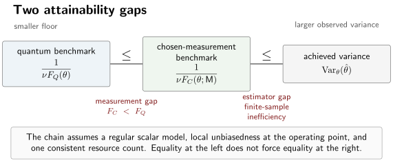
For a regular, locally unbiased scalar problem, $1/(\nu F_Q)\le1/(\nu F_C)\le\operatorname{Var}(\hat\theta)$. The first gap is caused by a measurement that does not extract all available state information; the second is caused by an inefficient estimator, finite data, or both. Either inequality may be strict.

Classical Scalar Theorem

Let $D$ denote the complete classical record with likelihood $p(D\mid\theta)$. Define the score and Fisher information by

$$U_\theta(D) = \partial_\theta\log p(D\mid\theta),$$ $$F_D(\theta) = \mathbb E_\theta[U_\theta^2].$$

Let $T(D)$ estimate $\theta$. If the model and estimator satisfy the regularity conditions below and $T$ is locally unbiased at $\theta_0$, then

$$\operatorname{Var}_{\theta_0}(T) \ge \frac{1}{F_D(\theta_0)}.$$

The bound uses the Fisher information of the entire record. If $D=(X_1,\ldots,X_\nu)$ consists of independent, identically distributed observations, then

$$F_D(\theta) = \nu F_1(\theta),$$

and

$$\operatorname{Var}_\theta(T) \ge \frac{1}{\nu F_1(\theta)}.$$

For correlated, adaptive, stopped, or postselected data, one must calculate the information of the correct joint likelihood rather than insert a nominal shot count into the independent formula.

Regularity Assumptions

A standard proof requires conditions such as:

1. The sample space and support do not change with $\theta$ in a way that creates unaccounted boundary terms.
2. The likelihood is differentiable in a neighborhood of the operating point.
3. Differentiation may be interchanged with summation or integration.
4. The score has finite second moment and $0<F_D(\theta_0)<\infty$.
5. The estimator has finite variance and the derivative of its mean exists.
6. The requested parameter direction is locally identifiable.

Under these assumptions,

$$\mathbb E_\theta[U_\theta] = \partial_\theta \int p(D\mid\theta)dD =0.$$

This zero-mean score identity is the hinge of the proof. If the support moves with $\theta$, differentiating the normalization integral can produce a boundary term, and the ordinary theorem may fail.

Regularity is not a decorative phrase. It is part of the result.

Proof by Cauchy–Schwarz

Write the estimator mean as

$$m(\theta) = \mathbb E_\theta[T].$$

Differentiating under the integral gives

$$\begin{aligned} m'(\theta) &= \int T(D)\, \partial_\theta p(D\mid\theta)dD\\ &= \mathbb E_\theta[TU_\theta]. \end{aligned}$$

Because $\mathbb E_\theta[U_\theta]=0$,

$$m'(\theta) = \mathbb E_\theta \left[ (T-m)U_\theta \right].$$

Cauchy–Schwarz now implies

$$[m'(\theta)]^2 \le \operatorname{Var}_\theta(T) F_D(\theta).$$

For a locally unbiased estimator, $m'(\theta_0)=1$, so

$$\operatorname{Var}_{\theta_0}(T) \ge \frac{1}{F_D(\theta_0)}.$$

The theorem is therefore a covariance inequality between the estimation error and the score. Fisher information appears because it is the score variance.

Global and Local Unbiasedness

An estimator is globally unbiased if

$$\mathbb E_\theta[T]=\theta$$

for every allowed $\theta$. It is locally unbiased at $\theta_0$ if

$$\mathbb E_{\theta_0}[T]=\theta_0, \qquad \left. \frac{d}{d\theta} \mathbb E_\theta[T] \right|_{\theta_0} =1.$$

Local unbiasedness is weaker and is the condition normally used in local quantum estimation. The estimator may be calibrated around one operating point without being unbiased over the whole parameter space.

For a periodic phase, ordinary global unbiasedness is often impossible. The mean of any estimator defined consistently on the circle is periodic, whereas the coordinate function $\theta$ on an unwrapped real line is not. A circular loss, a restricted prior interval, or a covariant phase criterion is then more appropriate than forcing the scalar theorem onto the wrong topology.

Equality and Efficient Estimators

Equality in Cauchy–Schwarz occurs only if the centered estimator is proportional to the score almost surely:

$$T(D)-m(\theta) = \frac{m'(\theta)}{F_D(\theta)} U_\theta(D).$$

For a globally unbiased estimator this becomes

$$T(D)-\theta = \frac{U_\theta(D)}{F_D(\theta)}.$$

The left side is a fixed function of the data, while the right side generally depends on the unknown parameter. Exact finite-sample equality is therefore special. Regular exponential-family models supply important examples.

Under standard identifiability, smoothness, and moment assumptions, a maximum likelihood estimator is often asymptotically efficient:

$$\sqrt\nu (\hat\theta_{\rm ML}-\theta) \xrightarrow{d} \mathcal N \left( 0, \frac{1}{F_1(\theta)} \right).$$

This is an asymptotic theorem, not a finite-sample guarantee. Boundary solutions, weak identification, multimodal likelihoods, and rare events can delay or destroy the approximation.

Exact Example: Bernoulli Data

Let $X_k\sim\operatorname{Bernoulli}(\theta)$ independently and define

$$\hat\theta = \bar X = \frac1\nu\sum_{k=1}^{\nu}X_k.$$

The estimator is unbiased and

$$\operatorname{Var}(\bar X) = \frac{\theta(1-\theta)}{\nu}.$$

One observation has

$$F_1(\theta) = \frac{1}{\theta(1-\theta)},$$

so

$$\frac{1}{\nu F_1(\theta)} = \frac{\theta(1-\theta)}{\nu}.$$

The sample proportion exactly attains the bound for interior values $0<\theta<1$. At the endpoints, the parameter lies on a boundary and the usual open-neighborhood regularity assumptions change.

Biased Estimators and Mean-Square Error

Define the bias

$$b(\theta) = \mathbb E_\theta[T]-\theta.$$

Then

$$m'(\theta)=1+b'(\theta),$$

and the same proof gives the biased Cramér–Rao inequality

$$\operatorname{Var}_\theta(T) \ge \frac{[1+b'(\theta)]^2}{F_D(\theta)}.$$

Variance alone no longer measures estimation error. The mean-square error is

$$\operatorname{MSE}_\theta(T) = \operatorname{Var}_\theta(T)+b(\theta)^2,$$

so

$$\operatorname{MSE}_\theta(T) \ge b(\theta)^2 + \frac{[1+b'(\theta)]^2}{F_D(\theta)}.$$

A biased estimator can have variance below the unbiased bound without violating anything. Shrinkage, clipping, regularization, and boundary projection deliberately trade variance for bias. They should be compared by the declared risk, not by variance alone.

Estimating a Function of the Parameter

If $T$ is unbiased for a differentiable function $g(\theta)$,

$$\mathbb E_\theta[T]=g(\theta),$$

then

$$\operatorname{Var}_\theta(T) \ge \frac{[g'(\theta)]^2}{F_D(\theta)}.$$

This form makes reparameterization transparent. If $\phi=g(\theta)$ is the estimand, the Fisher information in the $\phi$ coordinate is

$$F^{(\phi)} = F^{(\theta)} \left( \frac{d\theta}{d\phi} \right)^2,$$

and both expressions give the same physical variance bound after units are transformed consistently.

Multiparameter Classical Bound

For a parameter vector $\boldsymbol\theta=(\theta^1,\ldots,\theta^p)$, define the score vector and Fisher matrix

$$u_\mu(D) = \partial_\mu\log p(D\mid\boldsymbol\theta),$$ $$J_{\mu\nu} = \mathbb E [u_\mu u_\nu].$$

Let the estimator vector have mean $\mathbf m(\boldsymbol\theta)$ and Jacobian

$$B_{a\mu} = \partial_\mu m_a.$$

Under the matrix regularity assumptions,

$$\operatorname{Cov}(\hat{\mathbf g}) \succeq B J^{-1}B^{\mathsf T}.$$

For a locally unbiased estimator of $\boldsymbol\theta$ itself, $B=I$ and

$$\operatorname{Cov}(\hat{\boldsymbol\theta}) \succeq J^{-1}.$$

The ordering means that the difference is positive semidefinite. It does not mean every entry of the covariance matrix is separately greater than the corresponding entry of $J^{-1}$.

For a positive cost matrix $W$, the matrix inequality implies

$$\operatorname{Tr} \left[ W\operatorname{Cov}(\hat{\boldsymbol\theta}) \right] \ge \operatorname{Tr}(WJ^{-1}).$$

The weights carry units and encode which parameter combinations matter.

Nuisance Parameters and the Schur Complement

Partition the parameter vector into a scalar target $\alpha$ and nuisance parameters $\boldsymbol\lambda$:

$$J = \begin{pmatrix} J_{\alpha\alpha} & J_{\alpha\lambda}\\ J_{\lambda\alpha} & J_{\lambda\lambda} \end{pmatrix}.$$

If $J_{\lambda\lambda}$ is invertible, the effective information for $\alpha$ is the Schur complement

$$J_{\rm eff} = J_{\alpha\alpha} - J_{\alpha\lambda} J_{\lambda\lambda}^{-1} J_{\lambda\alpha}.$$

The target variance obeys

$$\operatorname{Var}(\hat\alpha) \ge \frac{1}{J_{\rm eff}} = (J^{-1})_{\alpha\alpha}.$$

If the nuisance parameters were known, the formal bound would instead be $1/J_{\alpha\alpha}$. Correlation between target and nuisance scores makes $J_{\rm eff}\le J_{\alpha\alpha}$, so unknown contrast, loss, background, phase offset, or calibration drift can substantially weaken a precision claim.

Singular Information and Constraints

A singular Fisher matrix means that at least one local parameter combination does not change the likelihood to first order. More data from the same design cannot identify a structurally null direction.

A Moore–Penrose pseudoinverse can express a bound only for gradients lying in the estimable tangent subspace. Applying $J^+$ mechanically to an unidentifiable target can produce a finite-looking number with no operational meaning. One should instead expose the null space, reparameterize to identifiable combinations, add measurements, or supply justified external calibration.

Known equality constraints reduce the tangent space. The correct constrained Cramér–Rao bound projects onto that tangent space; it is not obtained by inverting the unconstrained singular matrix and hoping the unwanted direction disappears.

When Regularity Fails

Consider $n$ independent samples from

$$X_k\sim\operatorname{Uniform}(0,\theta).$$

The support depends on $\theta$. Inside the support, $\partial_\theta\log p=-1/\theta$, whose expectation is not zero; the moving upper boundary supplies the term omitted by a naive differentiation under the integral.

The maximum $X_{(n)}$ gives the unbiased estimator

$$T = \frac{n+1}{n}X_{(n)},$$

with variance

$$\operatorname{Var}_\theta(T) = \frac{\theta^2}{n(n+2)}.$$

This can appear to beat a naively computed regular Cramér–Rao expression. The resolution is not super-efficiency or new physics: the theorem’s score identity is false for this moving-support model.

Irregular problems call for a theorem adapted to their structure, such as a finite-difference Hammersley–Chapman–Robbins or Barankin bound, not a repaired symbol inserted into the regular proof.

Scalar Quantum Cramér–Rao Bound

Let $\rho_\theta$ be a differentiable quantum-state family and $\mathsf M$ a parameter-independent POVM. The measurement produces a classical likelihood with information $F_C(\theta;\mathsf M)$, while the SLD quantum Fisher information satisfies

$$F_C(\theta;\mathsf M) \le F_Q(\theta).$$

For $\nu$ independent copies $\rho_\theta^{\otimes\nu}$,

$$F_Q (\rho_\theta^{\otimes\nu}) = \nu F_Q(\rho_\theta).$$

Any locally unbiased estimator built from any allowed joint measurement on those copies therefore obeys

$$\begin{aligned} \operatorname{Var}_\theta(\hat\theta) &\ge \frac{1}{F_C^{(\nu)}(\theta;\mathsf M)}\\ &\ge \frac{1}{\nu F_Q(\theta)}. \end{aligned}$$

The second line is the scalar SLD quantum Cramér–Rao bound. It is a bound on a declared state family and copy model. If the experiment optimizes entangled inputs across parameterized channel uses, controls, ancillas, or error correction, the QFI of the resulting complete strategy replaces the single-state expression.

Two Separate Attainability Questions

Reaching the quantum bound requires both inequalities in the chain to become equalities.

Measurement attainability

For a regular one-parameter model at a known operating point, measuring in an SLD eigenbasis extracts $F_Q$. The measurement can depend on the unknown $\theta$, however. A practical protocol may need a coarse first stage to localize the parameter and a second adaptive stage near the estimated operating point.

Estimator attainability

After a measurement is fixed, its classical bound is exactly attained only when the estimator error is proportional to the score. More commonly, a regular maximum likelihood or efficient estimator approaches the bound as the number of copies grows.

Thus an SLD-optimal measurement does not guarantee finite-sample equality, and an efficient estimator cannot recover information discarded by a poor measurement. The two gaps in the figure are logically independent.

Local Quantum Bounds and Global Error

For the equatorial qubit phase family

$$\lvert\psi_\theta\rangle = \frac{ \lvert0\rangle+e^{i\theta}\lvert1\rangle }{\sqrt2},$$

the QFI is $F_Q=1$, so the local bound for $\nu$ copies is

$$\operatorname{Var}_{\theta_0}(\hat\theta) \ge \frac1\nu.$$

This says nothing about choosing among phase branches separated by $2\pi$. With a broad prior, an estimator can have a narrow conditional peak near each branch and still make rare, large branch errors. Those threshold errors can dominate global mean-square risk while the local QFI remains unchanged.

The quantum Cramér–Rao bound can therefore be locally tight and globally optimistic at the same time. Dynamic range and prior localization are part of the task, not corrections to be appended after quoting the bound.

Multiparameter Quantum Bounds

For several parameters, the SLD quantum Fisher matrix $J_Q$ gives the formal matrix inequality

$$\operatorname{Cov}(\hat{\boldsymbol\theta}) \succeq \frac1\nu J_Q^{-1}.$$

Measurements that optimize different directions may be incompatible. The matrix can be mathematically valid as a lower bound while no one measurement attains all its entries simultaneously.

Commuting SLDs on the state support provide a strong compatibility condition. Weaker mean-commutator conditions can make the SLD cost asymptotically attainable in regular models with collective measurements. Outside compatible models, one should use a bound that includes the measurement tradeoff.

Holevo Cramér–Rao Bound

Fix an operating point and a positive weight matrix $W$. Consider Hermitian operators $X_\mu$ satisfying local unbiasedness constraints

$$\operatorname{Tr}(\rho X_\mu)=0,$$ $$\operatorname{Tr} \left[ (\partial_\nu\rho)X_\mu \right] = \delta_{\mu\nu}.$$

Define

$$Z_{\mu\nu}[\mathbf X] = \operatorname{Tr}(\rho X_\mu X_\nu).$$

The Holevo cost is

$$\begin{aligned} C_H(W) = \min_{\mathbf X} \bigg\{ &\operatorname{Tr} \left[W\operatorname{Re}Z\right]\\ &+ \left\| \sqrt W\operatorname{Im}Z\sqrt W \right\|_1 \bigg\}. \end{aligned}$$

In regular independent-copy models, it gives the asymptotically attainable weighted quantum limit

$$\operatorname{Tr} \left[ W\operatorname{Cov}(\hat{\boldsymbol\theta}) \right] \ge \frac{C_H(W)}{\nu}.$$

The SLD scalarized cost is

$$C_S(W) = \operatorname{Tr}(WJ_Q^{-1}),$$

and

$$C_H(W)\ge C_S(W).$$

The nonnegative trace-norm term penalizes incompatible imaginary cross-correlations. In compatible models the two costs coincide; otherwise the Holevo bound is tighter and reflects the price of joint estimation.

Do not confuse the Holevo Cramér–Rao bound with the Holevo bound on accessible classical information. They are different results. Also avoid the acronym “HCRB” without expansion: it is used for both the Holevo Cramér–Rao and Hammersley–Chapman–Robbins bounds.

Bayesian van Trees Inequality

Local unbiasedness may be inappropriate when the parameter has a meaningful prior distribution. Let $\pi(\theta)$ be a differentiable prior satisfying the boundary conditions needed for integration by parts. Its Fisher information is

$$I_\pi = \int \pi(\theta) \left[ \partial_\theta\log\pi(\theta) \right]^2d\theta.$$

For squared-error Bayes risk

$$R_B = \int \pi(\theta) \mathbb E_\theta \left[ (T-\theta)^2 \right]d\theta,$$

the scalar van Trees inequality gives

$$R_B \ge \frac{1}{ \int\pi(\theta)F_D(\theta)d\theta +I_\pi }.$$

For $\nu$ independent observations, $F_D=\nu F_1$. For a quantum-state family, pointwise $F_C\le F_Q$ yields the generally weaker but measurement-independent bound

$$R_B \ge \frac{1}{ \nu\int\pi(\theta)F_Q(\theta)d\theta +I_\pi }.$$

The prior term is information, not a free resource. A narrow prior can make the Bayes risk small before any measurement. Comparisons must use the same prior or charge the experiment that created it.

Exact Bayesian Example

Suppose

$$X_k\mid\theta \sim \mathcal N(\theta,\sigma^2), \qquad \theta\sim\mathcal N(0,\tau^2).$$

The data information and prior information are

$$F_D=\frac{\nu}{\sigma^2}, \qquad I_\pi=\frac1{\tau^2}.$$

The van Trees bound is

$$R_B \ge \left( \frac{\nu}{\sigma^2} + \frac1{\tau^2} \right)^{-1}.$$

The posterior mean has posterior variance

$$\operatorname{Var}(\theta\mid D) = \left( \frac{\nu}{\sigma^2} + \frac1{\tau^2} \right)^{-1},$$

independent of the observed values, so its Bayes risk attains the bound exactly. This example also makes clear that prior and data information add in this conjugate Gaussian model.

Finite-Difference and Global Alternatives

The ordinary Cramér–Rao theorem examines an infinitesimal parameter change. Finite-difference bounds compare separated hypotheses and can remain useful when derivatives, support, or global identifiability are troublesome.

For an unbiased estimator of $g(\theta)$, one Hammersley–Chapman–Robbins form is

$$\operatorname{Var}_\theta(T) \ge \sup_{\theta'\ne\theta} \frac{ [g(\theta')-g(\theta)]^2 }{ \mathbb E_\theta \left[ \left( \frac{p(D\mid\theta')}{p(D\mid\theta)}-1 \right)^2 \right] },$$

when the required absolute-continuity conditions hold. The denominator is a $\chi^2$ divergence. In a regular model, taking $\theta'\to\theta$ recovers the differential Cramér–Rao expression. The Barankin construction combines several alternative parameter points and gives the tightest variance lower bound within a broad unbiased class, but is often harder to evaluate.

Bayesian Ziv–Zakai and Weiss–Weinstein bounds connect estimation risk to binary discrimination at finite parameter separations. Their quantum versions replace classical testing performance by quantum state-discrimination limits. They are especially useful in threshold regimes where a local QFI predicts a narrow peak but rare branch errors dominate total risk.

These alternatives answer different questions. A tighter global bound is not a correction factor to the Cramér–Rao formula; it uses a broader view of the parameter space and usually different assumptions.

Postselection, Heralding, and Missing Events

Suppose an attempt succeeds with probability $q(\theta)$ and the success flag is recorded. The full Fisher information includes both the flag and the conditional records:

$$\begin{aligned} F_{\rm full} ={}& \frac{[\partial_\theta q]^2}{q(1-q)}\\ &+ qF_{\rm succ} + (1-q)F_{\rm fail}. \end{aligned}$$

A bound conditioned only on successful events uses $F_{\rm succ}$ and a random number of retained trials. It cannot be compared fairly with a per-attempt or per-time benchmark unless the success probability, failed attempts, waiting time, and stopping rule are restored to the resource model.

Parameter-dependent filtering can also bias the retained estimator. The appropriate Cramér–Rao form must use that bias and the likelihood of every reported and discarded category.

Adaptive and Correlated Records

For an adaptive experiment with history $H_{k-1}$, the joint likelihood factorizes conditionally:

$$p(D\mid\theta) = \prod_{k=1}^{\nu} p(x_k\mid H_{k-1},\theta).$$

Under regularity, conditional scores have zero conditional mean, so the total Fisher information is the expected sum of conditional informations:

$$F_D(\theta) = \sum_{k=1}^{\nu} \mathbb E_\theta \left[ F_k(\theta\mid H_{k-1}) \right].$$

This is not necessarily $\nu$ times one fixed number because the settings and conditional distributions change with the history. For genuinely correlated noise or latent drift, even this conditional model must include the shared variables. Applying an independent-shot bound to correlated data usually overstates information.

Variance Bounds Are Not Confidence Intervals

The Cramér–Rao inequality concerns repeated-sampling variance or an integrated Bayes risk. It does not provide:

• a confidence interval for the observed data set;
• guaranteed frequentist coverage;
• a posterior credible probability;
• a tail bound for rare errors;
• robustness to model misspecification;
• a calibration uncertainty budget.

An estimator can have variance near the bound and still have biased tails, poor coverage, or branch failures. Confidence procedures, posterior checks, bootstrap or likelihood diagnostics, and calibration propagation remain separate tasks.

Reporting a Quantum Precision Bound

A trustworthy report should state:

1. the estimand, units, domain, and operating point;
2. the complete state or channel model and the implemented POVM;
3. whether the quoted information is $F_C$, $F_Q$, or a channel-optimized quantity;
4. the copy, time, energy, loss, and postselection resource denominator;
5. the estimator and whether unbiasedness is local, global, or absent;
6. all nuisance parameters and the effective matrix bound;
7. whether the bound is finite-sample, asymptotic, Bayesian, or minimax;
8. measurement and estimator attainability evidence;
9. global ambiguity, boundary, and support checks;
10. achieved MSE, interval coverage, and calibration uncertainty alongside the theoretical floor.

The bound is useful precisely because it separates an information limit from implementation. Reporting both makes the gap scientifically interpretable.

Common Mistakes

• Quoting $1/F$ without saying whether $F$ is per shot or total.
• Applying the unbiased bound to a biased or clipped estimator and comparing variance instead of MSE.
• Assuming differentiation under the integral when support depends on the parameter.
• Treating local unbiasedness as global identifiability.
• Inverting a singular Fisher matrix without checking estimable directions.
• Ignoring nuisance parameters and using $1/J_{\alpha\alpha}$ instead of the Schur-complement result.
• Treating the SLD matrix bound as jointly attainable when optimal measurements are incompatible.
• Assuming an SLD-optimal POVM also supplies an efficient finite-sample estimator.
• Reporting a conditional postselection bound per success as if it were per attempted resource.
• Calling a variance lower bound a confidence interval or achieved precision.
• Using “HCRB” without distinguishing Holevo Cramér–Rao from Hammersley–Chapman–Robbins.
• Comparing bounds computed with different priors, time budgets, or parameter units.

Cross-Links

• Ramsey Interferometry applies local, nuisance-aware, and Bayesian bounds to a periodic binary likelihood with a finite capture range.
• Classical and Quantum Fisher Information derives the information quantities and measurement optimization used here.
• Fisher Information owns the score, additivity, curvature, and classical examples.
• Quantum Measurement as Estimation develops likelihood construction, estimators, uncertainty, and validation.
• Standard Quantum Limit applies the independent-copy quantum bound to resource scaling.
• Heisenberg Scaling shows when a quadratic local QFI becomes an inverse-resource error law and why global ambiguity or noise can change that conclusion.
• Variance and Covariance supplies the covariance and positive-semidefinite ordering used in matrix bounds.
• Bayes’ Rule gives the posterior identity underlying Bayes risk.
• Quantum Channels and Noise owns noisy channel models that must be included before computing a quantum bound.
• Sensing Case Studies shows how local bounds interact with calibration, bandwidth, and achieved evidence.
• Claims, Hype, and Evidence Standards supplies the broader resource and comparator audit.
• Quantum Information Roadmap places the theorem after the estimation model and Fisher metrics.

References

1. C. R. Rao, “Information and the accuracy attainable in the estimation of statistical parameters,” Bulletin of the Calcutta Mathematical Society 37, 81–91 (1945), reprint doi:10.1007/978-1-4612-0919-5_16.
2. H. Cramér, Mathematical Methods of Statistics, Princeton University Press (1946), publisher record.
3. E. L. Lehmann and G. Casella, Theory of Point Estimation, 2nd ed., Springer (1998), doi:10.1007/b98854.
4. S. M. Kay, Fundamentals of Statistical Signal Processing, Volume I: Estimation Theory, Prentice Hall (1993), publisher record.
5. H. L. Van Trees and K. L. Bell, Bayesian Bounds for Parameter Estimation and Nonlinear Filtering/Tracking, Wiley-IEEE Press (2007), doi:10.1002/0470120967.
6. R. D. Gill and B. Y. Levit, “Applications of the van Trees inequality: A Bayesian Cramér–Rao bound,” Bernoulli 1, 59–79 (1995), doi:10.2307/3318681.
7. J. M. Hammersley, “On estimating restricted parameters,” Journal of the Royal Statistical Society: Series B 12, 192–229 (1950), doi:10.1111/j.2517-6161.1950.tb00056.x.
8. D. G. Chapman and H. Robbins, “Minimum variance estimation without regularity assumptions,” Annals of Mathematical Statistics 22, 581–586 (1951), doi:10.1214/aoms/1177729548.
9. E. W. Barankin, “Locally best unbiased estimates,” Annals of Mathematical Statistics 20, 477–501 (1949), doi:10.1214/aoms/1177729943.
10. C. W. Helstrom, Quantum Detection and Estimation Theory, Academic Press (1976), doi:10.1016/C2013-0-10310-8.
11. A. S. Holevo, Probabilistic and Statistical Aspects of Quantum Theory, 2nd ed., Edizioni della Normale (2011), doi:10.1007/978-88-7642-378-9.
12. S. L. Braunstein and C. M. Caves, “Statistical distance and the geometry of quantum states,” Physical Review Letters 72, 3439–3443 (1994), doi:10.1103/PhysRevLett.72.3439.
13. M. G. A. Paris, “Quantum estimation for quantum technology,” International Journal of Quantum Information 7, 125–137 (2009), doi:10.1142/S0219749909004839.
14. A. Fujiwara and H. Nagaoka, “Quantum Fisher metric and estimation for pure state models,” Physics Letters A 201, 119–124 (1995), doi:10.1016/0375-9601(95)00327-J.
15. K. Matsumoto, “A new approach to the Cramér–Rao-type bound of the pure-state model,” Journal of Physics A 35, 3111–3123 (2002), doi:10.1088/0305-4470/35/13/307.
16. R. D. Gill and S. Massar, “State estimation for large ensembles,” Physical Review A 61, 042312 (2000), doi:10.1103/PhysRevA.61.042312.
17. O. E. Barndorff-Nielsen, R. D. Gill, and P. E. Jupp, “On quantum statistical inference,” Journal of the Royal Statistical Society: Series B 65, 775–816 (2003), doi:10.1111/1467-9868.00415.
18. J. Liu, H. Yuan, X.-M. Lu, and X. Wang, “Quantum Fisher information matrix and multiparameter estimation,” Journal of Physics A 53, 023001 (2020), doi:10.1088/1751-8121/ab5d4d.
19. F. Albarelli, J. F. Friel, and A. Datta, “Evaluating the Holevo Cramér–Rao bound for multiparameter quantum metrology,” Physical Review Letters 123, 200503 (2019), doi:10.1103/PhysRevLett.123.200503.
20. J. Yang, S. Pang, Y. Zhou, and A. N. Jordan, “Optimal measurements for quantum multiparameter estimation with general states,” Physical Review A 100, 032104 (2019), doi:10.1103/PhysRevA.100.032104.
21. M. Tsang, “Ziv–Zakai error bounds for quantum parameter estimation,” Physical Review Letters 108, 230401 (2012), doi:10.1103/PhysRevLett.108.230401.
22. S. D. Personick, “Application of quantum estimation theory to analog communication over quantum channels,” IEEE Transactions on Information Theory 17, 240–246 (1971), doi:10.1109/TIT.1971.1054643.
23. L. Seveso, M. A. C. Rossi, and M. G. A. Paris, “Quantum metrology beyond the quantum Cramér–Rao theorem,” Physical Review A 95, 012111 (2017), doi:10.1103/PhysRevA.95.012111.
24. R. Demkowicz-Dobrzański, M. Jarzyna, and J. Kołodyński, “Quantum limits in optical interferometry,” Progress in Optics 60, 345–435 (2015), doi:10.1016/bs.po.2015.02.003.

Exercises

1. Reconstruct the scalar proof

Let $T$ have mean $m(\theta)$ in a regular scalar model. Starting from the score, prove

$$\operatorname{Var}_\theta(T) \ge \frac{[m'(\theta)]^2}{F_D(\theta)}.$$

Solution

Regularity gives

$$\mathbb E[U_\theta]=0$$

and

$$m'(\theta) = \mathbb E[TU_\theta].$$

Subtracting $m\mathbb E[U_\theta]=0$ yields

$$m'(\theta) = \mathbb E[(T-m)U_\theta].$$

Cauchy–Schwarz gives

$$[m'(\theta)]^2 \le \mathbb E[(T-m)^2] \mathbb E[U_\theta^2] = \operatorname{Var}(T)F_D(\theta).$$

Rearranging proves the result. Local unbiasedness sets $m'(\theta_0)=1$.

2. Verify exact Bernoulli attainability

For $\nu$ independent Bernoulli trials, show that the sample proportion attains the Cramér–Rao bound for $0<\theta<1$.

Solution

The sample proportion satisfies

$$\mathbb E[\bar X]=\theta, \qquad \operatorname{Var}(\bar X) = \frac{\theta(1-\theta)}{\nu}.$$

One trial has information

$$F_1 = \frac1\theta+ \frac1{1-\theta} = \frac1{\theta(1-\theta)}.$$

Thus

$$\frac1{\nu F_1} = \frac{\theta(1-\theta)}{\nu} = \operatorname{Var}(\bar X).$$

3. Check a biased Gaussian estimator

Let $X\sim\mathcal N(\theta,\sigma^2)$ and $T=aX$ for a fixed real $a$. Compute its bias, variance, and biased Cramér–Rao bound.

Solution

The mean and bias are

$$m(\theta)=a\theta, \qquad b(\theta)=(a-1)\theta,$$

so $1+b'(\theta)=a$. The information is $F=1/\sigma^2$, and the biased bound is

$$\operatorname{Var}(T) \ge \frac{a^2}{1/\sigma^2} = a^2\sigma^2.$$

Because $\operatorname{Var}(aX)=a^2\sigma^2$, equality holds. The MSE is

$$\operatorname{MSE}(T) = a^2\sigma^2 + (a-1)^2\theta^2.$$

Reducing variance with $|a|<1$ does not remove the bias cost.

4. Diagnose the uniform-model failure

For $X_1,\ldots,X_n\sim\operatorname{Uniform}(0,\theta)$, explain which step of the ordinary proof fails and verify the variance of $T=(n+1)X_{(n)}/n$.

Solution

The support $0\le X_k\le\theta$ moves with the parameter. Differentiating the normalization integral while ignoring the moving boundary incorrectly gives a zero-mean score. Inside the support the joint log likelihood has derivative $-n/\theta$, whose expectation is not zero.

For the sample maximum,

$$\mathbb E[X_{(n)}] = \frac{n}{n+1}\theta,$$

and

$$\operatorname{Var}(X_{(n)}) = \frac{n\theta^2}{(n+1)^2(n+2)}.$$

Therefore $T$ is unbiased and

$$\operatorname{Var}(T) = \left(\frac{n+1}{n}\right)^2 \operatorname{Var}(X_{(n)}) = \frac{\theta^2}{n(n+2)}.$$

There is no contradiction because the regular Cramér–Rao theorem does not apply.

5. Compute a nuisance-parameter penalty

For one observation, let

$$J = \begin{pmatrix} 9&3\\ 3&4 \end{pmatrix},$$

where the first parameter is the target. Find its effective information and variance bound when the second parameter is unknown. Compare with the known-nuisance bound.

Solution

The Schur complement is

$$J_{\rm eff} = 9-3\left(\frac14\right)3 = \frac{27}{4}.$$

Thus for $\nu$ independent observations,

$$\operatorname{Var}(\hat\theta_1) \ge \frac{4}{27\nu}.$$

If the nuisance parameter were known, the bound would be

$$\frac{1}{9\nu}.$$

The unknown correlated parameter weakens the bound because $4/27>1/9$.

6. Separate quantum measurement and estimator gaps

A one-parameter qubit family has $F_Q=1$. An implemented measurement has $F_C=0.64$, and $\nu=100$ independent copies are used. Find the quantum floor and the measurement-specific classical floor. If the observed estimator variance is $0.020$, identify both gaps.

Solution

The quantum floor is

$$\frac1{\nu F_Q} = \frac1{100} =0.010.$$

The chosen-measurement floor is

$$\frac1{\nu F_C} = \frac1{64} =0.015625.$$

The difference between $0.010$ and $0.015625$ is the measurement gap. The difference between the classical floor $0.015625$ and the achieved variance $0.020$ is the estimator or finite-sample gap. The data obey

$$0.010 \le 0.015625 \le 0.020.$$

7. Saturate the Gaussian van Trees bound

Let $\theta\sim\mathcal N(0,4)$ and observe $\nu=3$ independent samples $X_k\mid\theta\sim\mathcal N(\theta,9)$. Compute the van Trees bound on Bayes MSE.

Solution

The data and prior informations are

$$F_D = \frac{3}{9} = \frac13, \qquad I_\pi = \frac14.$$

Hence

$$R_B \ge \frac{1}{1/3+1/4} = \frac{12}{7}.$$

The conjugate Gaussian posterior has variance $12/7$, so the posterior mean attains this Bayes-risk bound.

8. Recover Cramér–Rao from a finite difference

Assume a regular model and an unbiased estimator of $g(\theta)$. Show that the Hammersley–Chapman–Robbins expression tends to $[g'(\theta)]^2/F_D(\theta)$ as $\theta'=\theta+h$ and $h\to0$.

Solution

The numerator expands as

$$[g(\theta+h)-g(\theta)]^2 = h^2[g'(\theta)]^2+o(h^2).$$

For the likelihood ratio,

$$\frac{p(D\mid\theta+h)}{p(D\mid\theta)}-1 = hU_\theta(D)+o(h).$$

Therefore the denominator is

$$\mathbb E_\theta \left[ \left( \frac{p_{\theta+h}}{p_\theta}-1 \right)^2 \right] = h^2F_D(\theta)+o(h^2).$$

Taking the ratio and then the limit gives

$$\frac{[g'(\theta)]^2}{F_D(\theta)},$$

the scalar Cramér–Rao lower bound.