Magnetometry

A magnetometer estimates a specified property of a magnetic field from a physical response. In quantum magnetometry, that response is encoded in a quantum state or quantum dynamical process before a measurement produces classical data. The phrase “magnetic-field sensitivity” is incomplete until the field component, spatial weighting, temporal waveform, bandwidth, averaging convention, dynamic range, and operating conditions are stated.

This page is the canonical home for the platform-neutral quantum-estimation view of magnetometry. It develops the signal generator, likelihood, Fisher information, information rate, temporal filter, spatial mode, vector-field tradeoffs, quantum resources, and evidence needed to support a sensitivity or quantum-advantage claim.

Magnetometry in Atomic, Molecular, and Optical Physics owns optical pumping and readout, zero- and finite-field instruments, scalar and vector architectures, SERF operation, coil calibration, heading errors, systematic budgets, and application-level validation. Spin in Magnetic Fields owns the static spin Hamiltonian, sign conventions, and Zeeman spectrum. Dynamical Decoupling owns the detailed toggling-frame and filter-function derivations. The later NV-center case study specializes the framework to a solid-state spin sensor.

Start with the Estimand

A magnetic field is a vector field over space and time. A useful experiment rarely estimates all of it. Instead, it estimates one or several parameters in a model such as

$$\mathbf B(\mathbf r,t) = \mathbf B_0(\mathbf r,t) + b\,s(t)\mathbf u(\mathbf r) + \sum_a \nu_a\, s_a(t)\mathbf u_a(\mathbf r).$$

Here $b$ is the target parameter, $s(t)\mathbf u(\mathbf r)$ is its known spatiotemporal mode, and the $\nu_a$ are nuisance parameters. Depending on the task, $b$ might be

• a static field component at a calibrated location;
• the amplitude and phase of a sinusoidal field;
• a gradient or difference between two regions;
• a Fourier coefficient in a prescribed bandwidth;
• a source parameter inferred through a field model; or
• a stochastic quantity such as a power spectral density.

These are different statistical problems. A protocol optimized for a known sinusoid can reject a static offset and yet be a poor broadband magnetometer. A gradiometer can reject uniform environmental noise while being deliberately insensitive to the common field. A relaxometry experiment estimates noise near a transition frequency rather than a deterministic field amplitude.

The first line of a magnetometry specification should therefore state the estimand and the observation model. “Smallest detectable field” without this contract is not reproducible.

Magnetic Coupling as a Parameter Generator

Let a controlled sensor couple to an effective field component through

$$H_B(t) = -\hbar\gamma B(t)G,$$

where $\gamma$ is the signed gyromagnetic ratio and $G$ is a dimensionless generator. For a spin-$1/2$ sensor with quantization axis $z$, $G=\sigma_z/2$. For $N$ spins responding collectively,

$$G=J_z = \frac12\sum_{k=1}^{N}\sigma_z^{(k)}.$$

Suppose control pulses produce a toggling function $y(t)$ and the target field is $B(t)=b,s(t)$. If the effective generators commute at different times, the parameter-dependent unitary is

$$U_b = \exp\!\left(i\gamma b\mathcal A G\right), \qquad \mathcal A = \int_0^T y(t)s(t)\,dt.$$

The overlap $\mathcal A$ is the temporal signal gain. For a static field and free precession, $s(t)=y(t)=1$ and $\mathcal A=T$. A spin echo has equal positive and negative lobes, so it rejects a static field but can acquire phase from an alternating field synchronized to the sign changes.

For a pure input state, the quantum Fisher information (QFI) for $b$ is

$$F_b^{(Q)} = 4\gamma^2\mathcal A^2 \,(\Delta G)^2.$$

This equation separates three ingredients:

1. the coupling strength $|\gamma|$;
2. the temporal overlap $|\mathcal A|$; and
3. the generator variance supplied by the probe state.

It is a local bound for the specified parameter model. It does not by itself state the capture range, identify a realizable measurement, include cycle overhead, or guarantee robustness to nuisance fields.

A Binary Magnetometry Likelihood

Ramsey-like preparation and readout often produce a binary outcome $x\in\{+1,-1\}$ with likelihood

$$p(x\mid b) = \frac12 \left[ 1+xC\sin(\gamma b\mathcal A+\theta) \right].$$

The contrast $0\le C\le1$ includes imperfect preparation, dephasing, control errors, and readout visibility. The analysis phase $\theta$ selects the working point. The classical Fisher information is

$$F_b = \frac{ C^2\gamma^2\mathcal A^2 \cos^2(\gamma b\mathcal A+\theta) }{ 1-C^2\sin^2(\gamma b\mathcal A+\theta) }.$$

At quadrature, where the sine term vanishes,

$$F_b = C^2\gamma^2\mathcal A^2.$$

For $N$ independent, identically coupled spins read out in one cycle, the information adds:

$$F_{b,N} = NC^2\gamma^2\mathcal A^2.$$

The same scaling follows from the QFI. An equatorial coherent spin state has $(\Delta J_z)^2=N/4$, giving

$$F_b^{(Q)} = N\gamma^2\mathcal A^2$$

before contrast loss. Equality between a measurement’s classical Fisher information and the QFI requires the appropriate state, working point, and readout; quoting QFI alone does not establish experimental sensitivity.

Sensitivity Means Information per Wall Time

Let the complete cycle last

$$T_c = T+t_{\mathrm{prep}}+t_{\mathrm{read}}+t_{\mathrm{reset}}.$$

For statistically independent cycles at a fixed working point, the Fisher information rate is

$$\dot F_b = \frac{NC^2\gamma^2\mathcal A^2}{T_c}.$$

The corresponding local noise-equivalent field is

$$\eta_B \equiv \frac{1}{\sqrt{\dot F_b}} = \frac{\sqrt{T_c}} {C|\gamma|\,|\mathcal A|\sqrt N}.$$

For free-precession DC sensing, $\mathcal A=T$. Under the assumptions above, an averaging time $\tau=mT_c$ gives

$$\delta b(\tau) \ge \frac{\eta_B}{\sqrt\tau}.$$

The units of $\eta_B$ are $\mathrm{T}/\sqrt{\mathrm{Hz}}$, but numerical factors depend on one-sided versus two-sided spectral conventions and on how the estimator bandwidth is defined. A careful report supplies the convention rather than relying on the units to do that work.

Dead time matters twice. It reduces the number of trials per unit time, and it can expose a pulsed sensor to aliasing of environmental or local-oscillator noise. Rejected cycles, preparation failures, recalibration, and recovery from saturation belong in $T_c$ or in a separately reported duty factor.

Worked benchmark

Consider $N=10^6$ independent spins with

$$\frac{|\gamma|}{2\pi} = 7\,\mathrm{GHz/T}, \qquad T=1\,\mathrm{ms}, \qquad C=0.70, \qquad T_c=2\,\mathrm{ms}.$$

For a static field, $\mathcal A=T$, so the ideal projection-noise benchmark is

$$\begin{aligned} \eta_B &= \frac{\sqrt{2\times10^{-3}}} {0.70(2\pi)(7\times10^9)(10^{-3})\sqrt{10^6}} \\ &\simeq 1.45\times10^{-12} \ \mathrm{T}/\sqrt{\mathrm{Hz}}. \end{aligned}$$

This is not yet an instrument specification. It omits technical readout noise, field calibration, spatial averaging, correlated cycles, estimator loss, dynamic range, and uptime. Its value is that it states a transparent reference against which the complete device can be compared.

Temporal Modes and Filter Matching

Write the field along the sensed axis as

$$B(t)=b,s(t)+\xi_B(t),$$

where $s(t)$ is a deterministic target waveform and $\xi_B(t)$ is stationary zero-mean magnetic noise. The accumulated phase is

$$\phi = \gamma b\mathcal A + \gamma\int_0^T y(t)\xi_B(t)\,dt.$$

The control modulation $y(t)$ is therefore both a signal template and a noise filter. Define

$$Y(\omega) = \int_0^T y(t)e^{i\omega t}\,dt.$$

For a sinusoidal signal $s(t)=\cos(\omega_s t+\varphi_s)$,

$$\mathcal A = \operatorname{Re} \left[ e^{i\varphi_s}Y(\omega_s) \right].$$

With the two-sided power spectral density convention

$$\left\langle \widetilde\xi_B(\omega) \widetilde\xi_B^*(\omega') \right\rangle = 2\pi\delta(\omega-\omega')S_B(\omega),$$

the phase variance is

$$\operatorname{Var}(\phi_{\mathrm n}) = \gamma^2 \int_{-\infty}^{\infty} \frac{d\omega}{2\pi} S_B(\omega)|Y(\omega)|^2.$$

For Gaussian phase noise, the coherence is

$$C(T)=e^{-\chi(T)}, \qquad \chi(T) = \frac12\operatorname{Var}(\phi_{\mathrm n}).$$

Different spectral conventions move factors of two between $S_B$, $\chi$, and the integration range. The physical prediction is unchanged if one convention is used consistently.

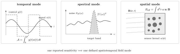
A magnetometer responds to a specified mode, not to an abstract field number. The temporal overlap $\mathcal A$ sets signal gain, the same filter samples the noise spectrum, and the spatial kernel $w(\mathbf r)$ defines the effective field. Sensitivity, bandwidth, and spatial resolution must be reported together.

Filter matching has a hard limitation: control cannot reject noise that is indistinguishable from the signal in the same spatiotemporal mode. More pulses can suppress low-frequency noise while sharpening an AC passband, but pulse errors, finite pulse duration, timing jitter, harmonics, and reduced duty factor can erase the expected gain. The ideal $Y(\omega)$ and the measured transfer function should both be reported.

Coherence and the Optimal Interrogation Time

Longer interrogation increases phase gain, but it usually reduces contrast. For a phenomenological stretched-exponential envelope,

$$C(T) = \exp\!\left[-(T/T_2)^p\right],$$

the DC information rate with negligible overhead is

$$\dot F_b(T) = N\gamma^2T \exp\!\left[-2(T/T_2)^p\right].$$

Its optimum satisfies

$$T_* = T_2 \left(\frac{1}{2p}\right)^{1/p}.$$

With fixed dead time $t_d$, the rate becomes

$$\dot F_b(T) = \frac{ N\gamma^2T^2e^{-2(T/T_2)^p} }{T+t_d},$$

and the stationary condition is

$$\frac2T - \frac{2pT^{p-1}}{T_2^p} - \frac1{T+t_d} =0.$$

This optimization is local and model-dependent. Phase wrapping may force a shorter $T$; overhead can favor a longer $T$; colored noise can invalidate the stretched-exponential model; and adaptive multi-time protocols can combine a wide capture range with a long final interrogation.

Bandwidth, Dynamic Range, and Aliasing

A single sensitivity number hides the sensor transfer function. At minimum, one should distinguish

• interrogation bandwidth: the width of the temporal filter around its target frequency;
• sampling bandwidth: limited by cycle time and irregular dead time;
• closed-loop bandwidth: relevant when feedback tracks a field;
• analysis bandwidth: imposed by the estimator or reported spectrum; and
• usable bandwidth: the region over which calibration, linearity, and noise are validated.

The binary likelihood is periodic in phase. For one interrogation, fields separated by

$$\Delta b_{mathrm{alias}} = \frac{2\pi}{|\gamma\mathcal A|}$$

produce the same ideal probability. A roughly linear single-fringe interval is smaller still. Increasing $T$ improves local sensitivity while reducing unambiguous range. Bias fields, quadrature readout, multiple interrogation times, adaptive control, and an independent coarse channel can resolve aliases, but those resources belong in the protocol description.

For a continuously operated linear sensor, it is often clearer to write

$$m(\omega) = \chi_{MB}(\omega)B_{\mathrm{eff}}(\omega) + n_M(\omega),$$

where $m$ is the measured output and $\chi_{MB}$ is the calibrated complex response. Output noise referred to the input gives

$$S_B^{\mathrm{eq}}(\omega) = \frac{S_M(\omega)}{|\chi_{MB}(\omega)|^2}.$$

An amplitude spectral density $\sqrt{S_B^{\mathrm{eq}}}$ has units $\mathrm{T}/\sqrt{\mathrm{Hz}}$; the PSD has units $\mathrm{T}^2/\mathrm{Hz}$; and a one-shot standard deviation has units $\mathrm T$. These quantities should not be interchanged.

Spatial Modes and Source Geometry

Real sensors average the field over a finite region. A scalar channel can be modeled as

$$B_{\mathrm{eff}}(t) = \int d^3r\, w(\mathbf r) \mathbf n(\mathbf r)\cdot \mathbf B(\mathbf r,t), \qquad \int d^3r\,w(\mathbf r)=1.$$

The kernel $w(\mathbf r)$ includes sensor density, optical intensity, mode overlap, collection efficiency, and analysis weighting. The local sensitive axis is $\mathbf n(\mathbf r)$. Two devices with the same field-noise floor can have very different value for a localized source because their active volumes, standoff distances, and kernels differ.

Spatial resolution is not simply the physical sensor size. It also depends on source distance, field propagation, channel geometry, inversion priors, and regularization. For a multi-channel array,

$$B_i(t) = \int d^3r\, \mathbf K_i(\mathbf r)\cdot \mathbf J_s(\mathbf r,t) +n_i(t),$$

where $\mathbf J_s$ denotes a source distribution and $\mathbf K_i$ is a forward kernel. Estimating the source is then an inverse problem, not merely a collection of independent field estimates. Cross-channel covariance and uncertainty in the kernels must enter the inference.

A gradiometer estimates a difference such as

$$g_B = \frac{B_1-B_2}{d}.$$

Common-mode rejection depends on matched gains, axes, transfer functions, and timing. A low differential noise floor does not establish the absolute noise of either channel.

Vector Magnetometry Is Multiparameter Estimation

For a spin coupled to all three components,

$$H_B = -\hbar\gamma \left( B_xJ_x+B_yJ_y+B_zJ_z \right).$$

Near a chosen operating point, a pure-state QFI matrix has the schematic form

$$F_{\mu\nu}^{(Q)} = 4\gamma^2T^2 \operatorname{Cov}_{\mathrm s}(J_\mu,J_\nu),$$

where

$$\operatorname{Cov}_{\mathrm s}(A,B) = \frac12\langle AB+BA\rangle - \langle A\rangle\langle B\rangle.$$

Unlike three unrelated scalar parameters, the field components are generated by noncommuting observables. Measurements that are optimal for different components need not be jointly compatible. The matrix quantum Cramér–Rao bound may therefore be unattainable by one measurement, even though each diagonal entry is attainable in a separate experiment.

Practical vector sensors address this by using distinct orientations, independent subensembles, sequential settings, controlled bias fields, or a joint measurement designed for a weighted cost. The resource split must be visible: three subensembles containing $N/3$ sensors do not each inherit the $N$-sensor scalar benchmark.

Nuisance fields also reduce information. If $b$ is the target and $\boldsymbol\nu$ collects unknown nuisance parameters, then for a classical Fisher matrix the effective local information is the Schur complement

$$F_{b,\mathrm{eff}} = F_{bb} - F_{b\nu} F_{\nu\nu}^{-1} F_{\nu b}.$$

Calibration data or prior information can improve this quantity, but they are then resources in the inference. Treating unknown transverse fields as known can make a scalar sensitivity estimate unrealistically optimistic.

What Quantum Resources Can Improve

For independent spins, generator variances add and the local QFI scales as $N$. This is the standard quantum limit for the matched preparation, interrogation, readout, and wall-time resources. Quantum correlations can change the variance or the accessible measurement noise.

Spin squeezing

For a collective spin used as a small-angle sensor, the Wineland parameter

$$\xi_R^2 = \frac{N(\Delta J_\perp)^2} {|\langle\mathbf J\rangle|^2}$$

gives an ideal phase variance

$$(\Delta\phi)^2 = \frac{\xi_R^2}{N}.$$

Thus $\xi_R^2<1$ can provide a constant-factor metrological gain. The useful quantity includes contrast, coupling inhomogeneity, state-preparation time, readout noise, and loss. Noise reduction in a detector quadrature without a calibrated signal response is not sufficient.

Maximally correlated probes

An ideal GHZ-like state has $(\Delta G)^2\propto N^2$ and can achieve local QFI proportional to $N^2$. It also produces a fringe $N$ times narrower, reducing the prior range, and is fragile to loss and dephasing. Under independent Markovian dephasing, optimizing interrogation time commonly removes the asymptotic scaling advantage even though finite-$N$ gains may remain. Claims about Heisenberg scaling must specify the noise model and count sequential queries, preparation, ancillas, control, and repetitions.

Measurement backaction and conditional gain

Continuous or repeated nondemolition readout can conditionally squeeze an ensemble and track a field at the same time. Probe photons or auxiliary modes then contribute imprecision, backaction, decoherence, and sample disturbance. An in-loop record can look quieter because feedback suppresses the measured quantity. Independent or out-of-loop validation is needed to show that the field estimate itself improved.

The strongest comparison is end to end: the quantum protocol and its best classical reference use the same sensing particles, active volume, total time, bandwidth, field mode, prior range, calibration information, accepted trials, and disturbance budget.

Energy Resolution per Bandwidth

Field sensitivity alone favors large sensing volumes. A common cross-platform normalization is the magnetic energy resolution per bandwidth

$$E_R = \frac{S_B V}{2\mu_0},$$

where $S_B$ is a field-noise PSD and $V$ is an effective sensor volume. Its units are energy times time, or action. The expression is motivated by the magnetic energy density $B^2/(2\mu_0)$.

This metric can reveal tradeoffs hidden by a bare field-noise floor, and many sensor classes operate near scales of order $\hbar$. It is not a universal single-number ranking or a geometry-free quantum limit. The appropriate $V$, spectral convention, measured component, bandwidth, demagnetizing geometry, coupling efficiency, and standoff must be defined. A nanoscale sensor and a large-volume ensemble may solve different source-estimation problems even when their $E_R$ values coincide.

A Complete Performance Contract

A defensible magnetometry result reports enough information to reconstruct the measurement task and comparison. A useful ledger includes:

1. Estimand: component, waveform, phase convention, spatial kernel, and nuisance parameters.
2. Coupling: signed $\gamma$, generator, bias field, sensor number, active volume, orientation, and standoff.
3. Protocol: preparation, control sequence, interrogation time, readout, reset, estimator, and feedback.
4. Transfer function: complex gain, passband, phase, sampling, latency, and nonlinearity over the claimed range.
5. Noise: raw spectra, spectral convention, correlations, drift, aliases, and a decomposition that keeps measured and subtracted noise distinct.
6. Quantum resource: state witness, contrast, detected fraction, failed preparations, overhead, and matched classical reference.
7. Spatial performance: kernel or point-spread model, resolution, array covariance, and uncertainty in source geometry.
8. Calibration: field source, traceability chain, gain uncertainty, cross-axis response, cross-talk, and recalibration schedule.
9. Robustness: dynamic range, overload recovery, uptime, environmental conditions, and sensitivity to model mismatch.
10. Evidence: raw-data policy, uncertainty propagation, preregistered or blinded comparisons where appropriate, and out-of-loop validation.

No single row can repair a missing row elsewhere. A sub-projection-noise spin measurement, for example, may establish a valuable state-level result without yet establishing a better deployed magnetometer.

Evidence Ladder

Magnetometry claims become stronger in stages:

1. State evidence: tomography, squeezing, entanglement, or generator variance demonstrates a potentially useful probe.
2. Response evidence: a calibrated field produces the predicted likelihood or transfer function.
3. Estimator evidence: repeated blind signals have calibrated bias, variance, and confidence-interval coverage.
4. Sensor evidence: the installed device improves input-referred noise at matched bandwidth, range, geometry, and wall time.
5. Task evidence: a source or scientific parameter is inferred better under realistic nuisance conditions.
6. Operational evidence: the gain survives drift, recalibration, downtime, and independent replication.

Each level is meaningful. The mistake is to describe evidence at one level as if the higher levels had already been demonstrated.

Common Mistakes

Reporting a field number without a mode

A sensitivity in $\mathrm{T}/\sqrt{\mathrm{Hz}}$ does not identify the sensed component, spatial average, target frequency, or estimator bandwidth. State all four.

Confusing coherence time with optimum sensing time

$T_2$ characterizes an envelope under a specified sequence. The optimum $T$ also depends on signal overlap, overhead, phase range, and the actual noise spectrum.

Treating a filter peak as a complete bandwidth

The ideal $|Y(\omega)|^2$ omits pulse errors, sampling aliases, electronics, feedback, and analysis filters. Validate the end-to-end complex response.

Comparing unequal spatial resources

Field noise improves with sensor number and volume, while source coupling can fall rapidly with standoff. Match geometry or explicitly model the source task.

Calling any below-shot-noise trace quantum advantage

Noise subtraction, conditioning, postselection, unequal duty factor, or a changed transfer function can lower a trace without improving unconditional field information. Compare calibrated estimators with all trials counted.

Ignoring vector nuisance parameters

Unknown transverse fields, axis errors, and gain cross-talk consume information. Include them in a multiparameter model or show experimentally that they are negligible.

Extrapolating local Fisher information across aliases

Fisher information describes local curvature of a likelihood. It does not guarantee a globally unique estimate or protection from phase slips.

Exercises

1. Independent-spin Fisher information

For $N$ independent spins with

$$p(x\mid b) = \frac12[1+xC\sin(\gamma bT)],$$

derive the Fisher information at $b=0$. What one-shot bound follows?

Solution

At $b=0$, both outcomes have probability $1/2$, and

$$\left.\partial_b p(x\mid b)\right|_{b=0} = \frac{xC\gamma T}{2}.$$

The single-spin Fisher information is

$$F_{b,1} = \sum_{x=\pm1} \frac{(C\gamma T/2)^2}{1/2} = C^2\gamma^2T^2.$$

Independent information adds, so

$$F_{b,N} = NC^2\gamma^2T^2.$$

The local Cramér–Rao bound for one cycle is

$$\delta b \ge \frac{1}{C|\gamma|T\sqrt N}.$$

2. Projection-noise benchmark

Reproduce the worked benchmark for $N=10^6$, $|\gamma|/(2\pi)=7\,\mathrm{GHz/T}$, $T=1\,\mathrm{ms}$, $C=0.70$, and $T_c=2\,\mathrm{ms}$. What uncertainty is expected after $100\,\mathrm s$ under the independent-cycle model?

Solution

The information-rate expression gives

$$\eta_B = 1.45\times10^{-12} \ \mathrm{T}/\sqrt{\mathrm{Hz}}.$$

After $\tau=100\,\mathrm s$,

$$\delta b(100\,\mathrm s) = \frac{\eta_B}{\sqrt{100}} \simeq 1.45\times10^{-13}\ \mathrm T.$$

This extrapolation assumes stationary, independent cycles and no drift floor. A real long-duration test must verify the $\tau^{-1/2}$ regime.

3. Optimize stretched-exponential coherence

With negligible dead time and $C(T)=e^{-(T/T_2)^p}$, derive the interrogation time that maximizes DC Fisher information per unit time. Evaluate $T_*/T_2$ for $p=1$ and $p=2$.

Solution

Apart from constants,

$$\dot F_b(T) \propto Te^{-2(T/T_2)^p}.$$

The logarithmic derivative is

$$\frac{d}{dT}\ln\dot F_b = \frac1T - \frac{2pT^{p-1}}{T_2^p}.$$

Setting it to zero gives

$$\left(\frac{T_*}{T_2}\right)^p = \frac1{2p},$$

so

$$\frac{T_*}{T_2} = \left(\frac1{2p}\right)^{1/p}.$$

Therefore $T_*/T_2=1/2$ for $p=1$ and $T_*/T_2=1/2$ for $p=2$. The equality for these two cases is coincidental.

4. Echo as a matched filter

Let

$$y(t) = \begin{cases} +1,&0\le t<T/2,\\ -1,&T/2\le t\le T. \end{cases}$$

Find $\mathcal A$ for a static signal $s(t)=1$. Then find it for a signal that changes sign at $T/2$ in synchrony with $y(t)$.

Solution

For the static signal,

$$\mathcal A = \int_0^{T/2}dt - \int_{T/2}^{T}dt =0.$$

The echo rejects an ideal static field. For the synchronized signal $s(t)=y(t)$,

$$\mathcal A = \int_0^T y^2(t)\,dt =T.$$

The same sequence can therefore reject one temporal mode and retain another. This is mode selection, not universal noise suppression.

5. Local sensitivity and capture range

A protocol has $|\gamma\mathcal A|=2\pi\times10^6\,\mathrm{T}^{-1}$. Find the field spacing between equivalent fringes. What happens to this spacing if the interrogation overlap doubles?

Solution

The alias spacing is

$$\Delta b_{\mathrm{alias}} = \frac{2\pi}{|\gamma\mathcal A|} = 10^{-6}\ \mathrm T.$$

Doubling $|\mathcal A|$ doubles the local phase response and Fisher information amplitude, but halves the fringe spacing to $0.5\,\mu\mathrm T$. The local precision improves while the unambiguous range shrinks.

6. A nuisance field

The Fisher matrix for target field $b$ and nuisance offset $\nu$ is

$$F = \begin{pmatrix} 100&60\\ 60&50 \end{pmatrix} \mathrm T^{-2}.$$

Find the effective information about $b$ when $\nu$ is unknown. Compare it with the value obtained by pretending $\nu$ were known.

Solution

The Schur complement is

$$F_{b,\mathrm{eff}} = 100- \frac{60^2}{50} =28\ \mathrm T^{-2}.$$

The corresponding local variance bound is $1/28\,\mathrm T^2$, rather than $1/100\,\mathrm T^2$. Correlation with an unknown nuisance parameter removes most of the nominal information about $b$.

7. Energy resolution per bandwidth

A sensor has one-sided field-noise PSD $S_B=10^{-30}\,\mathrm{T^2/Hz}$ and effective volume $V=1.0\,\mathrm{mm^3}$. Estimate $E_R/\hbar$ using $\mu_0=4\pi\times10^{-7}\,\mathrm{H/m}$ and $\hbar=1.055\times10^{-34}\,\mathrm{J,s}$.

Solution

Since $1\,\mathrm{mm^3}=10^{-9}\,\mathrm{m^3}$,

$$E_R = \frac{10^{-30}\times10^{-9}} {2(4\pi\times10^{-7})} \simeq 3.98\times10^{-34}\ \mathrm{J,s}.$$

Thus

$$\frac{E_R}{\hbar} \simeq 3.8.$$

The number is meaningful only with the stated spectral and effective-volume conventions. It does not determine spatial resolution or source sensitivity.

8. Audit a quantum-enhanced magnetometer

An experiment reports $5\,\mathrm{dB}$ of squeezing and a lower magnetic-noise spectrum after subtracting photon shot noise. List at least eight additional items needed for an unconditional device-level quantum-advantage claim.

Solution

A defensible audit should include at least:

1. a calibrated magnetic-field response for squeezed and reference protocols;
2. the full input-referred spectrum without noise subtraction;
3. matched sensor number, active volume, standoff, and field mode;
4. preparation, readout, reset, and total cycle time;
5. all trials, including failed preparations and postselection;
6. contrast and coupling inhomogeneity in the metrological squeezing parameter;
7. bandwidth, transfer-function phase, dynamic range, and alias behavior;
8. estimator bias and uncertainty coverage on blind injected fields;
9. technical-noise covariance and drift over the claimed averaging interval;
10. calibration uncertainty and cross-axis response;
11. an independent or out-of-loop validation channel; and
12. a matched best classical strategy under the same disturbance and uptime constraints.

The squeezing measurement can already be scientifically important. The extra evidence is what connects state quality to unconditional sensor performance.

References

1. D. Budker and M. Romalis, “Optical magnetometry,” Nature Physics 3, 227–234 (2007).
2. C. L. Degen, F. Reinhard, and P. Cappellaro, “Quantum sensing,” Reviews of Modern Physics 89, 035002 (2017).
3. M. W. Mitchell and S. Palacios Alvarez, “Colloquium: Quantum limits to the energy resolution of magnetic field sensors,” Reviews of Modern Physics 92, 021001 (2020).
4. M. Koschorreck, M. Napolitano, B. Dubost, and M. W. Mitchell, “Sub-projection-noise sensitivity in broadband atomic magnetometry,” Physical Review Letters 104, 093602 (2010).
5. V. G. Lucivero, R. Jiménez-Martínez, J. Kong, and M. W. Mitchell, “Squeezing-enhanced optical magnetometry,” Physical Review Letters 116, 163603 (2016).
6. R. J. Sewell, M. Koschorreck, M. Napolitano, B. Dubost, N. Behbood, and M. W. Mitchell, “Magnetic sensitivity beyond the projection noise limit by spin squeezing,” Physical Review Letters 109, 253605 (2012).
7. S. F. Huelga, C. Macchiavello, T. Pellizzari, A. K. Ekert, M. B. Plenio, and J. I. Cirac, “Improvement of frequency standards with quantum entanglement,” Physical Review Letters 79, 3865–3868 (1997).
8. M. Tsang, H. M. Wiseman, and C. M. Caves, “Fundamental quantum limit to waveform estimation,” Physical Review Letters 106, 090401 (2011).
9. T. Baumgratz and A. Datta, “Quantum enhanced estimation of a multidimensional field,” Physical Review Letters 116, 030801 (2016).
10. J. F. Barry et al., “Sensitivity optimization for NV-diamond magnetometry,” Reviews of Modern Physics 92, 015004 (2020).
11. L. Pezzè, A. Smerzi, M. K. Oberthaler, R. Schmied, and P. Treutlein, “Quantum metrology with nonclassical states of atomic ensembles,” Reviews of Modern Physics 90, 035005 (2018).

Further Connections

• Instrument Magnetometry develops atomic and optical architectures, pumping and readout, SERF operation, calibrated vector response, systematic errors, and applications.
• Quantum Measurement as Estimation develops likelihoods, estimators, loss functions, priors, nuisance parameters, and evidence levels.
• Classical and Quantum Fisher Information owns the information inequalities and attainability conditions used here.
• Ramsey Interferometry develops the binary fringe, working-point control, phase aliases, adaptive schedules, and information per wall time.
• Spin Squeezing develops collective-spin covariance, the Wineland parameter, entanglement witnesses, readout noise, and end-to-end gain.
• Standard Quantum Limit defines the matched independent-sensor benchmark and separates constant improvement from scaling claims.
• Heisenberg Scaling treats correlated probes, prior width, sequential queries, noise, and resource counting.
• Dynamical Decoupling derives toggling functions, filter functions, pulse-sequence passbands, and control imperfections.
• Noise Spectra defines spectral-density conventions, stationarity, and quantum versus classical noise.
• NV Centers and Solid-State Defects introduces the NV Hamiltonian, optical preparation and readout, dephasing, and relaxometry.
• NV-Center Sensing applies the framework to photon-count likelihoods, CW and pulsed protocols, spatial transfer, vector reconstruction, and nanoscale NMR.
• Sensing Case Studies compares magnetometers, clocks, interferometers, and electrometers under shared evidence standards.