Entanglement Measures

Short Definition

An entanglement measure assigns a nonnegative number to a quantum state relative to a specified subsystem split and a specified class of free operations. In bipartite resource theory, the free states are separable states and the usual free operations are local operations and classical communication (LOCC). A useful measure must therefore not increase when the parties use only LOCC.

That sentence does not define one universal number. It defines a contract for a family of quantities. Entanglement entropy answers the reversible asymptotic question for pure bipartite states. Concurrence gives a special closed route to two-qubit entanglement of formation. Negativity is computable but misses positive-partial-transpose entanglement. Distillable entanglement asks what can be extracted, while entanglement of formation asks what a decomposition costs. Squashed entanglement has strong structural properties but requires a difficult optimization over extensions.

The measure must be chosen for the state class, partition, allowed operations, copy regime, and operational question. Equal values of one measure do not generally make two states interchangeable, and no single scalar captures all bipartite mixed-state or multipartite entanglement structure.

This page owns that selection problem in quantum information. The mathematical derivations remain at Entanglement Entropy, Concurrence for Two Qubits, and Negativity and PPT Criterion.

Start with the Operational Contract

Before computing a number, record six pieces of information.

1. Subsystem structure: Which tensor factors, modes, spatial regions, or operator algebras define the parties?
2. Partition: Is the question about $A\vert B$, $A\vert BC$, every bipartition, or genuine multipartite entanglement?
3. State class: Is the global state pure or mixed, finite dimensional or continuous variable, exactly known or inferred from data?
4. Free operations: Are the parties allowed one-way LOCC, two-way LOCC, separable operations, or the larger class of PPT-preserving operations?
5. Copy regime: Is the task single-copy, one-shot with an error tolerance, or asymptotic over many independent copies?
6. Task: Is the goal detection, state preparation, Bell-pair extraction, communication, conversion, comparison, or a computable bound?

Changing any one of these can change the correct measure. Even the phrase “the entanglement of $\rho$” is incomplete until the split is stated.

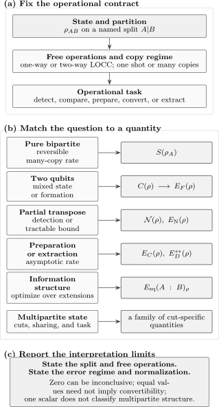
Choose a measure only after fixing the partition, state class, allowed operations, copy regime, and task. The right column names useful quantities, not interchangeable definitions of a single universal scalar.

What Makes a Quantity an Entanglement Measure?

Let $E(\rho_{AB})$ be a candidate bipartite quantity. Conventions differ, but the following properties organize most of the literature.

Vanishing on free states

Every separable state should have zero entanglement:

$$\begin{aligned} \rho_{AB} &= \sum_x p_x\, \rho_A^{(x)}\otimes\rho_B^{(x)} \\ &\Longrightarrow E(\rho_{AB})=0. \end{aligned}$$

If the converse also holds, the measure is faithful. Faithfulness is valuable but not universal among operational rates. Distillable entanglement, for example, vanishes on bound-entangled states even though those states are not separable.

Monotonicity under LOCC

For a deterministic LOCC channel $\Lambda$,

$$E\!\left(\Lambda(\rho_{AB})\right) \leq E(\rho_{AB}).$$

A stronger branch-resolved requirement applies to an LOCC instrument with outcome probabilities $p_i$ and normalized conditional states $\rho_i$:

$$E(\rho_{AB}) \geq \sum_i p_i E(\rho_i).$$

One postselected branch may have more entanglement than the input. The average cannot. Reporting only the successful branch while omitting its probability violates the operational accounting.

Local-unitary invariance follows because a local unitary and its inverse are both LOCC:

$$E\!\left( (U_A\otimes U_B)\rho_{AB} (U_A^\dagger\otimes U_B^\dagger) \right) =E(\rho_{AB}).$$

Desirable properties are not identical

Several additional properties are useful, but they answer different mathematical or operational concerns.

• Normalization: often $E(\Phi_d)=\log_2 d$ for a maximally entangled state of Schmidt rank $d$.
• Convexity: forgetting a classical preparation label should not increase the reported amount,

$$E\!\left(\sum_x p_x\rho_x\right) \leq \sum_x p_x E(\rho_x).$$

• Additivity: independent resources satisfy

$$E(\rho\otimes\sigma) = E(\rho)+E(\sigma).$$

• Asymptotic continuity: small state errors should not cause an extensive jump after the quantity is scaled by system size.
• Computability: a definition should admit an exact formula, controlled numerical optimization, or certified bounds in the intended setting.

These properties do not come as one package. Logarithmic negativity is additive and monotone under a broad class of operations, but it is not convex. Entanglement of formation is convex, but its optimization is generally hard. An operational rate can be conceptually exact while computationally inaccessible.

Measures at a Glance

Quantity	Natural domain	Main question	Main limitation
Entropy of entanglement	Pure bipartite states	Reversible asymptotic conversion rate	Reduced-state entropy is not a mixed-state measure
Concurrence	Two qubits	Closed mixed-state proxy and route to $E_F$	The Wootters formula is special to two qubits
Negativity $\mathcal N$	Bipartite mixed states	Computable NPT-sensitive quantifier	Vanishes on PPT entangled states
Logarithmic negativity $E_{\mathrm N}$	Bipartite and many continuous-variable settings	Additive computable bound on distillation	PPT blind and not convex
Entanglement of formation $E_F$	Bipartite mixed states	Least average pure-state entanglement in a decomposition	Convex-roof optimization is usually hard
Entanglement cost $E_C$	Asymptotic bipartite preparation	Bell pairs consumed per target copy	Requires regularization
Distillable entanglement $E_D$	Asymptotic bipartite extraction	Bell pairs recoverable per noisy copy	Depends on communication class and is often unknown
Squashed entanglement $E_{\mathrm{sq}}$	Bipartite states	Additive information-theoretic monotone and bounds	Optimization over all extensions is hard

The Entanglement Diagnostic Table answers a neighboring question: how to establish that entanglement is present. Detection criteria, witnesses, and Bell tests are not automatically quantitative measures.

Entropy of Entanglement

For a pure bipartite state $\lvert\psi\rangle_{AB}$, define

$$\rho_A = \operatorname{Tr}_B \lvert\psi\rangle\langle\psi\rvert.$$

The entropy of entanglement is

$$E(\psi) = S(\rho_A) = S(\rho_B),$$

with base-$2$ entropy

$$S(\rho) = -\operatorname{Tr} \left(\rho\log_2\rho\right).$$

If the Schmidt probabilities are $\lambda_k$, then

$$E(\psi) = -\sum_k\lambda_k\log_2\lambda_k.$$

It is zero for a product state and equals $\log_2 d$ for a maximally entangled state with $d$ equal Schmidt probabilities. For pure bipartite states in the many-copy, vanishing-error limit, this entropy gives both the rate at which Bell pairs can be distilled and the rate needed to create the state. This reversibility is why one number is so successful in that restricted setting.

Two cautions matter.

First, the full Schmidt spectrum, not only its entropy, governs deterministic single-copy LOCC conversion through majorization. Two pure states with equal entropy need not be exactly interconvertible in one shot.

Second, if $\rho_{AB}$ is mixed, $S(\rho_A)$ includes local thermal uncertainty, noise, and classical correlation. It is not a general mixed-state entanglement measure. A maximally mixed product state already has nonzero subsystem entropy and zero entanglement.

The canonical derivation and examples are at Entanglement Entropy and Schmidt Decomposition.

Concurrence

Concurrence is especially useful for two qubits. For

$$\lvert\psi\rangle = a\lvert00\rangle +b\lvert01\rangle +c\lvert10\rangle +d\lvert11\rangle,$$

the pure-state concurrence is

$$C(\psi) = 2\lvert ad-bc\rvert.$$

For a mixed two-qubit state, define the spin-flipped operator

$$\widetilde\rho = (\sigma_y\otimes\sigma_y) \rho^* (\sigma_y\otimes\sigma_y).$$

If $\lambda_1\geq\lambda_2\geq\lambda_3\geq\lambda_4$ are the square roots of the eigenvalues of $\rho\widetilde\rho$, then

$$C(\rho) = \max\!\left\{ 0,\, \lambda_1-\lambda_2-\lambda_3-\lambda_4 \right\}.$$

For two qubits, $C=0$ exactly for separable states and $C=1$ for Bell states. It also determines entanglement of formation:

$$E_F(\rho) = h_2\!\left( \frac{1+\sqrt{1-C(\rho)^2}}{2} \right),$$

where

$$h_2(x) = -x\log_2x -(1-x)\log_2(1-x).$$

This closed relation is exceptional. Generalized concurrences exist, but they are not one universal continuation of the two-qubit formula. A reported concurrence should always state the system dimension and definition. The derivation, spin-flip conventions, and worked Werner-state calculation belong to Concurrence for Two Qubits.

Negativity and Logarithmic Negativity

Take the partial transpose with respect to $B$:

$$\langle i\mu\rvert \rho^{T_B} \lvert j\nu\rangle = \langle i\nu\rvert \rho \lvert j\mu\rangle.$$

The trace norm is

$$\lVert X\rVert_1 = \operatorname{Tr} \sqrt{X^\dagger X}.$$

Negativity and logarithmic negativity are

$$\mathcal N(\rho) = \frac{ \lVert\rho^{T_B}\rVert_1-1 }{2},$$ $$E_{\mathrm N}(\rho) = \log_2 \lVert\rho^{T_B}\rVert_1 = \log_2\!\left(2\mathcal N+1\right).$$

Negativity is the absolute sum of the negative eigenvalues of $\rho^{T_B}$. A nonzero value therefore certifies entanglement. For a $d$-dimensional maximally entangled pair,

$$\mathcal N(\Phi_d) = \frac{d-1}{2}, \qquad E_{\mathrm N}(\Phi_d) = \log_2 d.$$

The logarithmic form is additive because the trace norm is multiplicative on tensor products. It also upper-bounds distillable entanglement under the corresponding asymptotic operational assumptions.

The limitation is structural, not numerical. Every state with positive partial transpose has

$$\mathcal N=E_{\mathrm N}=0.$$

In $2\times2$ and $2\times3$ systems, PPT is equivalent to separability. In higher dimensions, PPT entangled states exist, so zero negativity does not prove separability. Partial transpose is a diagnostic transformation, not a physical channel. See Negativity and PPT Criterion for the derivation and dimensional theorem.

Formation, Cost, and Distillation

Entanglement of formation

For a mixed state, consider every pure-state ensemble

$$\rho_{AB} = \sum_i p_i \lvert\psi_i\rangle\langle\psi_i\rvert.$$

Entanglement of formation is the convex roof

$$E_F(\rho_{AB}) = \inf_{\{p_i,\psi_i\}} \sum_i p_i\, S\!\left(\rho_A^{(i)}\right),$$

where

$$\rho_A^{(i)} = \operatorname{Tr}_B \lvert\psi_i\rangle\langle\psi_i\rvert.$$

The infimum is essential because a density operator has many ensemble decompositions. $E_F$ asks for the least average pure-state entanglement compatible with the mixed state, not the entanglement of one preferred preparation story.

Entanglement cost

The asymptotic Bell-pair cost is the regularized quantity

$$E_C(\rho) = \lim_{n\to\infty} \frac{1}{n} E_F\!\left(\rho^{\otimes n}\right).$$

Thus $E_F$ is a single-block convex-roof quantity, while $E_C$ is the many-copy preparation rate. They should not be silently identified.

Distillable entanglement

Suppose an LOCC protocol converts $n$ copies of $\rho$ into $m_n$ nearly perfect Bell pairs, with the error tending to zero as $n\to\infty$. The distillable entanglement is the best achievable rate:

$$E_D(\rho) = \sup_{\{\Lambda_n\}} \liminf_{n\to\infty} \frac{m_n}{n}.$$

The notation must specify whether $\Lambda_n$ permits one-way or two-way classical communication. Those rates can differ.

For bipartite pure states,

$$E_D(\psi) = E_C(\psi) = S(\rho_A).$$

For mixed states, formation and extraction can be irreversible:

$$0 \leq E_D(\rho) \leq E_C(\rho).$$

Some entangled mixed states have $E_D=0$ and are called bound entangled. Consequently, distillable entanglement is operationally sharp but not faithful. Exact values of $E_D$ are unknown for many ordinary-looking state families, so computable upper and lower bounds are often the scientifically honest result.

Entanglement Distillation owns the concrete BBPSSW recurrence, Bell-diagonal error map, hashing protocol, and finite-round success-and-yield ledger. Those protocols provide achievable lower bounds; this page retains the definition and comparison of the optimized measure.

Squashed Entanglement

An extension of $\rho_{AB}$ is any state $\rho_{ABE}$ satisfying

$$\operatorname{Tr}_E\rho_{ABE} = \rho_{AB}.$$

Squashed entanglement minimizes conditional mutual information over every such extension:

$$E_{\mathrm{sq}}(A:B)_\rho = \frac{1}{2} \inf_{\rho_{ABE}} I(A:B\mid E)_\rho,$$

where

$$\begin{aligned} I(A:B\mid E) ={}& S(AE)+S(BE) \\ &-S(E)-S(ABE). \end{aligned}$$

The extension asks how much of the observed $A$–$B$ correlation can be explained by a third system. The infimum removes correlation that can be mediated through $E$ and retains an irreducibly quantum contribution.

In finite dimensions, squashed entanglement is LOCC monotone, convex, additive, asymptotically continuous, monogamous, and faithful. It reduces to entanglement entropy on pure states. It also lies between important operational quantities:

$$E_D(\rho) \leq E_{\mathrm{sq}}(\rho) \leq E_F(\rho).$$

Its principal weakness is computability. The optimization ranges over extensions with no immediately fixed auxiliary dimension, and exact values are known only in restricted settings. Squashed entanglement is often most useful as a theorem-building quantity or a source of certified bounds, not as a routine number extracted from tomography.

Worked Comparison: A Noisy Bell Pair

Consider the two-qubit singlet mixed with white noise:

$$\rho_W(p) = p\lvert\Psi^-\rangle \langle\Psi^-\rvert + (1-p)\frac{I_4}{4}.$$

Here $0\leq p\leq1$.

Both reduced states are maximally mixed:

$$\rho_A=\rho_B=\frac{I_2}{2}.$$

Therefore $S(\rho_A)=1$ for every $p$. If subsystem entropy were misused as a mixed-state entanglement measure, it would claim that the maximally mixed state at $p=0$ has the same entanglement as the singlet at $p=1$.

The partial transpose has one potentially negative eigenvalue:

$$\mu_{\min} = \frac{1-3p}{4}.$$

Hence

$$\mathcal N(\rho_W) = \max\!\left\{ 0,\frac{3p-1}{4} \right\},$$

and

$$E_{\mathrm N}(\rho_W) = \log_2 \left( 1+2\mathcal N(\rho_W) \right).$$

The concurrence is

$$C(\rho_W) = \max\!\left\{ 0,\frac{3p-1}{2} \right\}.$$

Both quantities detect the same two-qubit entanglement threshold,

$$p>\frac{1}{3},$$

but their numerical scales differ. Concurrence can be inserted into the two-qubit formula for $E_F$; logarithmic negativity instead supplies an additive computable upper bound on distillation. Neither number is “the true amount” independently of the question.

For $p>1/3$, this two-qubit state is NPT and distillable, but the exact asymptotic distillation rate is not given by either $C$ or $\mathcal N$. This is typical: detection can be easy while operational rate calculation remains hard.

Choosing a Measure in Practice

If the state is pure and bipartite

Use the Schmidt spectrum first. Use entanglement entropy for asymptotic reversible rates, Rényi entropies for spectrum-sensitive comparisons and many-body scaling, and the full majorization relation for exact deterministic single-copy conversion.

If the state is an arbitrary two-qubit density operator

Use concurrence when the question is tied to two-qubit entanglement of formation. Use negativity when a partial-transpose calculation or comparison with larger local dimensions is more natural. Report the convention and do not compare the raw scales as though they used the same normalization.

If the state is higher dimensional and mixed

Negativity is a tractable NPT-sensitive quantity, not a complete detector. Entanglement of formation, cost, distillation, and squashed entanglement are operationally or structurally stronger but usually require optimization, regularization, or bounds. A positive witness or negative partial transpose certifies entanglement; failure of one detector does not settle separability.

If the task is resource conversion

Name the input and output units, error criterion, direction of classical communication, and asymptotic limit. Use $E_C$ for preparation cost and $E_D$ for extractable Bell-pair yield. A monotone that is easy to compute can provide a converse bound without equaling the achievable rate.

If the state comes from an experiment

Separate four claims:

1. the data reject all separable models allowed by the analysis;
2. a reconstructed density matrix is physical within uncertainty;
3. a chosen measure is bounded away from zero with stated confidence;
4. the measured resource supports a particular protocol at a quantified rate or fidelity.

These claims require different assumptions. Entanglement Witnesses can avoid full tomography, but a witness expectation is not automatically a calibrated entanglement amount. Tomographic plug-in estimates can be biased by finite samples and physicality constraints; report uncertainty and estimator assumptions.

Multipartite Cautions

For three or more parties, begin by naming a partition. The same state can have different entanglement across $A\vert BC$, $B\vert AC$, $C\vert AB$, and reduced two-party states.

For the GHZ state,

$$\lvert\mathrm{GHZ}\rangle = \frac{ \lvert000\rangle+\lvert111\rangle }{\sqrt2},$$

the entropy across every one-versus-two split is one bit. Yet every two-qubit reduced state is separable:

$$\rho_{AB} = \frac{1}{2} \left( \lvert00\rangle\langle00\rvert + \lvert11\rangle\langle11\rvert \right).$$

Pairwise concurrence therefore vanishes even though the global state has genuine tripartite entanglement.

For the W state,

$$\lvert W\rangle = \frac{ \lvert001\rangle +\lvert010\rangle +\lvert100\rangle }{\sqrt3},$$

two-party reductions retain pairwise entanglement. GHZ and W states are inequivalent under stochastic LOCC, and one scalar cannot encode that distinction, every bipartition, pairwise sharing, genuine multipartite structure, and conversion behavior simultaneously.

Multipartite work should report a family of quantities: entropies or negativities across named cuts, reduced-state measures, separability class, witnesses, and task-specific monotones. See Multipartite Systems, GHZ States, W States, and Monogamy of Entanglement.

Continuous Variables and Indistinguishable Particles

In continuous-variable systems, logarithmic negativity is popular because Gaussian partial transpose can be analyzed through covariance matrices. Entropies and trace norms may nevertheless require finite-energy assumptions, domain control, or converged truncations. Always specify the mode decomposition, quadrature convention, logarithm base, and cutoff treatment. The canonical entry points are Two-Mode Entanglement and Gaussian States Preview.

For identical particles, particle labels do not automatically define operational subsystems. Entanglement may instead refer to modes, orbitals, regions, or commuting observable algebras. Exchange symmetry alone is not a usable resource measure. See Identical-Particle Entanglement Cautions.

Common Mistakes

• Computing $S(\rho_A)$ for a mixed global state and calling it entanglement entropy without qualification.
• Reporting a measure without naming the subsystem split.
• Treating nonzero mutual information as proof of entanglement.
• Concluding that zero negativity implies separability in arbitrary dimension.
• Using concurrence outside the stated two-qubit convention.
• Calling $E_F$ the exact asymptotic preparation cost without regularization.
• Treating a distillation upper bound as an achievable rate.
• Ignoring whether classical communication is one-way or two-way.
• Reporting a successful filtering branch without its probability.
• Comparing raw values from differently normalized measures.
• Treating a witness, Bell violation, purity, or fidelity as a general entanglement measure.
• Compressing multipartite structure into one bipartition or one scalar.
• Quoting a numerical value without estimator uncertainty, cutoff convergence, or state-validity checks.

Connections

• Information-Theoretic Foundations determines whether the task needs a state diagnostic, entropy, entanglement measure, operational conversion claim, or a different canonical owner.
• Resource Theories owns the general conversion ledger and the distinction between a monotone bound and a complete criterion; this page retains entanglement-specific measure selection.
• Density Operators for Quantum Information supplies the state, partial-trace, fidelity, and numerical-validity workflow used here.
• Separable Mixed States owns the structural boundary between free and entangled bipartite states.
• LOCC Preview explains the free operations behind monotonicity.
• Entanglement Distillation turns Bell-diagonal error checks into explicit recurrence and hashing protocols while tracking accepted fidelity and resource yield together.
• Entanglement in Quantum Information connects Bell pairs, teleportation, dense coding, distillation, networks, and error correction.
• Classical Correlation versus Entanglement separates total correlation from nonseparability.
• Mutual Information develops a total-correlation quantity that should not be mistaken for an entanglement measure.
• Entanglement Diagnostic Table provides a quick setting-by-setting detection guide.

References

1. C. H. Bennett, H. J. Bernstein, S. Popescu, and B. Schumacher, “Concentrating Partial Entanglement by Local Operations”, Physical Review A 53, 2046–2052 (1996).
2. C. H. Bennett, D. P. DiVincenzo, J. A. Smolin, and W. K. Wootters, “Mixed-State Entanglement and Quantum Error Correction”, Physical Review A 54, 3824–3851 (1996).
3. G. Vidal, “Entanglement Monotones”, Journal of Modern Optics 47, 355–376 (2000).
4. W. K. Wootters, “Entanglement of Formation of an Arbitrary State of Two Qubits”, Physical Review Letters 80, 2245–2248 (1998).
5. A. Peres, “Separability Criterion for Density Matrices”, Physical Review Letters 77, 1413–1415 (1996).
6. G. Vidal and R. F. Werner, “A Computable Measure of Entanglement”, Physical Review A 65, 032314 (2002).
7. M. B. Plenio, “Logarithmic Negativity: A Full Entanglement Monotone That Is Not Convex”, Physical Review Letters 95, 090503 (2005).
8. M. Christandl and A. Winter, “Squashed Entanglement: An Additive Entanglement Measure”, Journal of Mathematical Physics 45, 829–840 (2004).
9. F. G. S. L. Brandão, M. Christandl, and J. Yard, “Faithful Squashed Entanglement”, Communications in Mathematical Physics 306, 805–830 (2011).
10. M. B. Plenio and S. Virmani, “An Introduction to Entanglement Measures”, Quantum Information and Computation 7, 1–51 (2007).
11. R. Horodecki, P. Horodecki, M. Horodecki, and K. Horodecki, “Quantum Entanglement”, Reviews of Modern Physics 81, 865–942 (2009).
12. V. Coffman, J. Kundu, and W. K. Wootters, “Distributed Entanglement”, Physical Review A 61, 052306 (2000).
13. W. Dür, G. Vidal, and J. I. Cirac, “Three Qubits Can Be Entangled in Two Inequivalent Ways”, Physical Review A 62, 062314 (2000).
14. E. Chitambar and G. Gour, “Quantum Resource Theories”, Reviews of Modern Physics 91, 025001 (2019).
15. J. Watrous, The Theory of Quantum Information, Cambridge University Press (2018).

Exercises

1. Normalization on a Bell pair. For $\lvert\Phi^+\rangle=(\lvert00\rangle+\lvert11\rangle)/\sqrt2$, calculate entanglement entropy, concurrence, negativity, logarithmic negativity, and entanglement of formation. What are $E_C$ and $E_D$ in the asymptotic pure-state setting?

Solution

Tracing out either qubit gives

$$\rho_A=\frac{I_2}{2},$$

so

$$S(\rho_A)=1.$$

For amplitudes $a=d=1/\sqrt2$ and $b=c=0$,

$$C=2\lvert ad-bc\rvert=1.$$

The partial transpose has eigenvalues

$$\left\{ \frac12,\frac12,\frac12,-\frac12 \right\},$$

hence

$$\mathcal N=\frac12, \qquad E_{\mathrm N} = \log_2(1+2\mathcal N) =1.$$

The Wootters relation gives $E_F=1$. Pure-state entanglement manipulation is asymptotically reversible, so

$$E_C=E_D=1$$

ebit per copy. The raw negativity is $1/2$, illustrating that normalization conventions differ even when the measures agree operationally on maximality.

2. A partially entangled pair. Let

$$\lvert\psi_\lambda\rangle = \sqrt{\lambda}\lvert00\rangle + \sqrt{1-\lambda}\lvert11\rangle.$$

Take $0\leq\lambda\leq1$. Find $E$, $C$, $\mathcal N$, and $E_{\mathrm N}$. Check the product and maximally entangled limits.

Solution

The Schmidt probabilities are $\lambda$ and $1-\lambda$, so

$$E(\psi_\lambda) = h_2(\lambda).$$

The concurrence is

$$C(\psi_\lambda) = 2\sqrt{\lambda(1-\lambda)}.$$

The partial-transpose eigenvalues are

$$\begin{gathered} \lambda,\quad 1-\lambda,\quad \sqrt{\lambda(1-\lambda)}, \\ -\sqrt{\lambda(1-\lambda)}. \end{gathered}$$

Therefore

$$\mathcal N(\psi_\lambda) = \sqrt{\lambda(1-\lambda)},$$

and

$$E_{\mathrm N}(\psi_\lambda) = \log_2 \left( 1+2\sqrt{\lambda(1-\lambda)} \right).$$

At $\lambda=0$ or $1$, all four quantities vanish. At $\lambda=1/2$,

$$E=C=E_{\mathrm N}=1, \qquad \mathcal N=\frac12.$$

The measures order this one-parameter pure-state family consistently, but their numerical scales are not the same.

3. The subsystem-entropy trap. For the noisy singlet $\rho_W(p)$ in the worked comparison, derive the potentially negative eigenvalue of $\rho_W^{T_B}$, the negativity, and the concurrence threshold. Explain why $S(\rho_A)$ fails.

Solution

The partial transpose of the singlet projector has eigenvalues

$$\frac12,\quad \frac12,\quad \frac12,\quad -\frac12.$$

Adding white noise shifts each eigenvalue by $(1-p)/4$ and multiplies the singlet contribution by $p$. Three eigenvalues become $(1+p)/4$, while the fourth is

$$\mu_{\min} = \frac{1-p}{4} -\frac{p}{2} = \frac{1-3p}{4}.$$

Thus

$$\mathcal N = \max\!\left\{ 0,\frac{3p-1}{4} \right\}.$$

The two-qubit concurrence formula gives

$$C = \max\!\left\{ 0,\frac{3p-1}{2} \right\}.$$

Both become positive exactly when $p>1/3$. However,

$$\rho_A=\frac{I_2}{2}$$

for every $p$, so $S(\rho_A)=1$ even at $p=0$, where $\rho_W=I_4/4$ is separable. The marginal entropy measures local mixedness, not mixed-state entanglement.

4. Additivity of logarithmic negativity. Use trace-norm multiplicativity to prove that $E_{\mathrm N}$ is additive on tensor products.

Solution

Partial transpose distributes over tensor products:

$$(\rho\otimes\sigma)^{T_{BB'}} = \rho^{T_B}\otimes\sigma^{T_{B'}}.$$

For finite trace-class operators,

$$\lVert X\otimes Y\rVert_1 = \lVert X\rVert_1 \lVert Y\rVert_1.$$

Therefore

$$\begin{aligned} E_{\mathrm N}(\rho\otimes\sigma) &= \log_2 \left\lVert \rho^{T_B}\otimes\sigma^{T_{B'}} \right\rVert_1 \\ &= \log_2 \left( \lVert\rho^{T_B}\rVert_1 \lVert\sigma^{T_{B'}}\rVert_1 \right) \\ &= E_{\mathrm N}(\rho) + E_{\mathrm N}(\sigma). \end{aligned}$$

Negativity itself is not additive because the affine transformation between $\mathcal N$ and $E_{\mathrm N}$ converts products of trace norms into

$$\begin{aligned} 1+2\mathcal N(\rho\otimes\sigma) &= \left(1+2\mathcal N(\rho)\right) \\ &\quad\times \left(1+2\mathcal N(\sigma)\right). \end{aligned}$$

5. Squashed entanglement of a pure state. Show that $E_{\mathrm{sq}}(A:B)_\psi=S(\rho_A)$ when $\rho_{AB}=\lvert\psi\rangle\langle\psi\rvert$ is pure.

Solution

Any extension of a pure state on $AB$ must factor:

$$\rho_{ABE} = \lvert\psi\rangle\langle\psi\rvert_{AB} \otimes\sigma_E.$$

Consequently,

$$\begin{aligned} S(AE)&=S(A)+S(E),\\ S(BE)&=S(B)+S(E),\\ S(ABE)&=S(E). \end{aligned}$$

Substitution into conditional mutual information gives

$$\begin{aligned} I(A:B\mid E) &= S(A)+S(B) \\ &= 2S(A), \end{aligned}$$

because a pure bipartite state has $S(A)=S(B)$. Every extension gives the same value, so the infimum does too:

$$E_{\mathrm{sq}}(A:B)_\psi = \frac12 I(A:B\mid E) = S(\rho_A).$$

6. Pairwise versus genuine tripartite entanglement. Trace out qubit $C$ from the GHZ state. Show that $\rho_{AB}$ is separable even though the entropy across $A\vert BC$ is one bit. What does this demonstrate about multipartite measures?

Solution

The GHZ projector contains two diagonal terms and two coherence terms:

$$\begin{aligned} \rho_{\mathrm{GHZ}} = \frac12\big( & \lvert000\rangle\langle000\rvert + \lvert111\rangle\langle111\rvert \\ & + \lvert000\rangle\langle111\rvert + \lvert111\rangle\langle000\rvert \big). \end{aligned}$$

The off-diagonal terms vanish under $\operatorname{Tr}_C$ because $\langle0\vert1\rangle=0$. Hence

$$\rho_{AB} = \frac12 \left( \lvert00\rangle\langle00\rvert + \lvert11\rangle\langle11\rvert \right),$$

which is an explicit convex mixture of product states. Its concurrence and negativity are zero.

By contrast,

$$\rho_A=\frac{I_2}{2}, \qquad S(\rho_A)=1,$$

so the pure global state has one ebit across $A\vert BC$. Pairwise measures can therefore vanish while genuine global entanglement remains. Multipartite characterization must name partitions and usually requires several quantities or a separability class, not one scalar.