Bloch Sphere

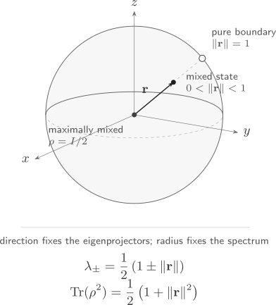
This is the canonical Bloch-sphere and Bloch-ball treatment, unifying pure spinors, mixed-qubit density operators, measurements, and rotation geometry. The density-operator application bridge is Bloch Sphere for Mixed States.

For a single qubit, the full state space of density operators is exactly the closed unit ball in $\mathbb R^3$. Every state has a unique representation

$$\rho = \frac12 \left( I+\mathbf r\cdot\boldsymbol\sigma \right), \qquad \lVert\mathbf r\rVert\leq1,$$

where

$$\boldsymbol\sigma = (X,Y,Z)$$

is the Pauli triple and $\mathbf r$ is the Bloch vector. Pure states lie on the unit sphere, mixed states lie in the interior, and the maximally mixed state $I/2$ sits at the center.

Pauli coordinates of a qubit state

The matrices $I,X,Y,Z$ are an orthogonal basis of the complex $2\times2$ matrices under the Hilbert–Schmidt inner product. Their trace identities are

$$\operatorname{Tr}\sigma_i=0, \qquad \operatorname{Tr}(\sigma_i\sigma_j) = 2\delta_{ij},$$

where $\sigma_i\in\{X,Y,Z\}$. Consequently, any Hermitian operator $H$ on a qubit can be expanded as

$$H = \frac12\operatorname{Tr}(H)\,I + \frac12 \sum_{i=x,y,z} \operatorname{Tr}(H\sigma_i)\sigma_i.$$

For a density operator, $\operatorname{Tr}\rho=1$, so

$$\rho = \frac12 \left( I+\sum_i r_i\sigma_i \right), \qquad r_i = \operatorname{Tr}(\rho\sigma_i).$$

Thus the three coordinates are directly the expectation values of the three Pauli observables:

$$\mathbf r = \left( \langle X\rangle_\rho, \langle Y\rangle_\rho, \langle Z\rangle_\rho \right).$$

Each $r_i$ is real. Indeed,

$$\begin{aligned} \left[ \operatorname{Tr}(\rho\sigma_i) \right]^* &= \operatorname{Tr} \left[ (\rho\sigma_i)^\dagger \right] \\ &= \operatorname{Tr}(\sigma_i\rho) \\ &= \operatorname{Tr}(\rho\sigma_i). \end{aligned}$$

The last step uses cyclicity of the trace. The Bloch vector is therefore not extra data attached to $\rho$; it is the same state expressed in a Pauli-adapted real coordinate system.

From matrix entries to the vector

Using

$$\begin{aligned} X &= \begin{pmatrix} 0&1\\ 1&0 \end{pmatrix}, \\[6pt] Y &= \begin{pmatrix} 0&-i\\ i&0 \end{pmatrix}, \\[6pt] Z &= \begin{pmatrix} 1&0\\ 0&-1 \end{pmatrix}. \end{aligned}$$

the Bloch form becomes

$$\rho = \frac12 \begin{pmatrix} 1+r_z&r_x-ir_y\\ r_x+ir_y&1-r_z \end{pmatrix}.$$

Conversely, write a trace-one Hermitian matrix as

$$\rho = \begin{pmatrix} a&c\\ c^*&1-a \end{pmatrix}.$$

Then

$$\begin{aligned} r_x&=2\operatorname{Re}c,\\ r_y&=-2\operatorname{Im}c,\\ r_z&=2a-1. \end{aligned}$$

The minus sign in $r_y$ follows from the displayed convention for $Y$. It is a frequent source of sign errors when one reads the off-diagonal entry without first fixing the Pauli convention.

Positivity makes a ball

Hermiticity and trace one do not by themselves make a matrix a physical state. Positivity supplies the geometric restriction. The Pauli product identity gives

$$(\mathbf r\cdot\boldsymbol\sigma)^2 = \lVert\mathbf r\rVert^2 I.$$

Therefore $\mathbf r\cdot\boldsymbol\sigma$ has eigenvalues $\pm\lVert\mathbf r\rVert$, and the eigenvalues of $\rho$ are

$$\lambda_\pm = \frac12 \left( 1\pm\lVert\mathbf r\rVert \right).$$

Because $\lambda_+\ge0$ automatically, positivity is equivalent to

$$\lambda_-\ge0 \qquad\Longleftrightarrow\qquad \lVert\mathbf r\rVert\leq1.$$

In matrix coordinates, the same condition can be written

$$\lvert c\rvert^2 \leq a(1-a), \qquad 0\leq a\leq1.$$

Indeed,

$$\det\rho = a(1-a)-\lvert c\rvert^2 = \frac14 \left( 1-\lVert\mathbf r\rVert^2 \right).$$

For a trace-one Hermitian $2\times2$ matrix, nonnegative determinant and nonnegative diagonal entries are equivalent to positive semidefiniteness. The unit-ball condition packages these constraints into one basis-independent statement.

The Bloch ball is the state space of one qubit. Direction selects a Pauli axis and eigenbasis; radius fixes the eigenvalues, purity, and determinant.

Spectrum: radius and direction

Let

$$r=\lVert\mathbf r\rVert.$$

When $r>0$, define the unit vector

$$\hat{\mathbf r} = \frac{\mathbf r}{r}$$

and the two rank-one projectors

$$P_\pm(\hat{\mathbf r}) = \frac12 \left( I\pm \hat{\mathbf r}\cdot\boldsymbol\sigma \right).$$

The spectral decomposition is then

$$\rho = \frac{1+r}{2} P_+(\hat{\mathbf r}) + \frac{1-r}{2} P_-(\hat{\mathbf r}).$$

This separates two roles:

• the direction $\hat{\mathbf r}$ fixes the eigenprojectors;
• the radius $r$ fixes the eigenvalues.

All states on a sphere of fixed radius have the same spectrum. They therefore have the same purity and von Neumann entropy, although they predict different outcomes for a fixed measurement axis. At the center $r=0$, the eigenvalues are degenerate and no direction or eigenbasis is preferred.

Pure states on the surface

Squaring the Bloch form gives

$$\rho^2 = \frac14 \left[ \left( 1+r^2 \right)I + 2\mathbf r\cdot\boldsymbol\sigma \right].$$

Taking the trace,

$$\operatorname{Tr}(\rho^2) = \frac12 \left( 1+r^2 \right).$$

For a normalized finite-dimensional state, purity is equivalent to $\operatorname{Tr}(\rho^2)=1$. Hence

$$\rho\ \text{is pure} \qquad\Longleftrightarrow\qquad r=1.$$

Every boundary point is a rank-one projector,

$$\rho = P_+(\hat{\mathbf r}) = \frac12 \left( I+\hat{\mathbf r}\cdot\boldsymbol\sigma \right).$$

For example,

$$\begin{aligned} \lvert0\rangle\langle0\rvert &= \frac12(I+Z), \\ \lvert1\rangle\langle1\rvert &= \frac12(I-Z), \\ \lvert+\rangle\langle+\rvert &= \frac12(I+X), \\ \lvert+i\rangle\langle+i\rvert &= \frac12(I+Y). \end{aligned}$$

The corresponding vectors are

$$\begin{aligned} \lvert0\rangle&\longleftrightarrow(0,0,1), & \lvert1\rangle&\longleftrightarrow(0,0,-1), \\ \lvert+\rangle&\longleftrightarrow(1,0,0), & \lvert+i\rangle&\longleftrightarrow(0,1,0). \end{aligned}$$

Antipodal surface points represent orthogonal pure states, not the same ray. For a unit vector $\hat{\mathbf n}$,

$$P_+(\hat{\mathbf n}) P_+(-\hat{\mathbf n}) = 0.$$

Angular parameterization

Up to a global phase, every pure qubit state can be written

$$\lvert\psi(\theta,\phi)\rangle = \cos\frac{\theta}{2}\lvert0\rangle + e^{i\phi} \sin\frac{\theta}{2}\lvert1\rangle.$$

Its projector has Bloch vector

$$\mathbf r = \left( \sin\theta\cos\phi, \sin\theta\sin\phi, \cos\theta \right).$$

The half-angle in the state vector and full angle on the sphere reflect the spinor geometry developed in the spin and symmetry treatment. For the density operator, the global phase has already disappeared.

Mixed states inside the ball

A qubit state is mixed exactly when

$$0\leq r<1.$$

Every interior point has two strictly positive eigenvalues and therefore rank two. Its purity lies in the interval

$$\frac12 \leq \operatorname{Tr}(\rho^2) < 1.$$

The lower endpoint occurs only at the center,

$$\mathbf r=\mathbf0, \qquad \rho_*=\frac I2.$$

This is the maximally mixed qubit state. It is invariant under every unitary transformation:

$$U\rho_*U^\dagger = \frac I2.$$

It also gives zero expectation value for every Pauli direction:

$$\operatorname{Tr} \left( \rho_*\, \hat{\mathbf n}\cdot\boldsymbol\sigma \right) = 0.$$

The center has no preferred eigenbasis. That fact is stronger than merely saying that its $Z$-basis populations are equal.

Mixtures are convex combinations

Suppose a preparation chooses $\rho_k$ with probability $p_k$. If $\rho_k$ has Bloch vector $\mathbf r_k$, then

$$\begin{aligned} \rho &= \sum_k p_k\rho_k, \\ \mathbf r &= \sum_k p_k\mathbf r_k. \end{aligned}$$

Statistical mixing is therefore ordinary convex averaging in the Bloch ball. A mixture of two states lies on the line segment joining their vectors.

For example, mixing the two antipodal pure states along $\hat{\mathbf n}$ gives

$$\begin{aligned} \rho &= pP_+(\hat{\mathbf n}) + (1-p)P_-(\hat{\mathbf n}), \\ \mathbf r &= (2p-1)\hat{\mathbf n}. \end{aligned}$$

At $p=1/2$ this becomes

$$\frac I2 = \frac12P_+(\hat{\mathbf n}) + \frac12P_-(\hat{\mathbf n})$$

for every direction $\hat{\mathbf n}$. The same center point therefore has infinitely many ensemble decompositions. More generally, an interior point lies on infinitely many chords of the sphere and admits many pure-state ensembles. The vector $\mathbf r$ determines the density operator, not which ensemble was used to prepare it; that distinction is treated in Ensembles and Preparation Procedures.

The radius is consequently not a unique “amount of classical ignorance.” It determines spectral mixedness, but it does not record a preparation history.

Measurement predictions

Pauli measurement along an axis

For a unit vector $\hat{\mathbf n}$, define

$$\sigma_{\hat{\mathbf n}} = \hat{\mathbf n}\cdot\boldsymbol\sigma.$$

Its eigenvalues are $\pm1$, with projectors

$$P_\pm(\hat{\mathbf n}) = \frac12 \left( I\pm \hat{\mathbf n}\cdot\boldsymbol\sigma \right).$$

Applying the trace rule gives

$$p_\pm = \operatorname{Tr} \left[ \rho P_\pm(\hat{\mathbf n}) \right] = \frac12 \left( 1\pm \mathbf r\cdot\hat{\mathbf n} \right).$$

Therefore

$$\begin{aligned} \left\langle \sigma_{\hat{\mathbf n}} \right\rangle_\rho &= \mathbf r\cdot\hat{\mathbf n}, \\ \operatorname{Var}_\rho \left( \sigma_{\hat{\mathbf n}} \right) &= 1- \left( \mathbf r\cdot\hat{\mathbf n} \right)^2. \end{aligned}$$

Geometrically, the measurement reads the signed projection of the Bloch vector onto the measurement axis. A pure state aligned with the axis has a deterministic outcome. The center gives $p_+=p_-=1/2$ along every axis.

Arbitrary qubit observable

Every Hermitian qubit observable has the form

$$A = a_0I+\mathbf a\cdot\boldsymbol\sigma, \qquad a_0\in\mathbb R, \quad \mathbf a\in\mathbb R^3.$$

Its eigenvalues are

$$a_\pm = a_0\pm\lVert\mathbf a\rVert.$$

The expectation value and variance are

$$\begin{aligned} \langle A\rangle_\rho &= a_0+\mathbf a\cdot\mathbf r, \\ \operatorname{Var}_\rho(A) &= \lVert\mathbf a\rVert^2 - \left( \mathbf a\cdot\mathbf r \right)^2. \end{aligned}$$

When $\mathbf a\ne\mathbf0$, the two measurement projectors point along $\pm\hat{\mathbf a}$, where

$$\hat{\mathbf a} = \frac{\mathbf a}{\lVert\mathbf a\rVert}.$$

The identity component $a_0I$ shifts both outcomes but changes neither their projectors nor the variance.

Worked diagnostics

A physical mixed state

Consider

$$\rho = \begin{pmatrix} \dfrac34&\dfrac{1-i}{4}\\[4pt] \dfrac{1+i}{4}&\dfrac14 \end{pmatrix}.$$

Reading off the components gives

$$\mathbf r = \left( \frac12, \frac12, \frac12 \right), \qquad r=\frac{\sqrt3}{2}.$$

Because $r<1$, the matrix is physical and mixed. Its eigenvalues and purity are

$$\lambda_\pm = \frac{2\pm\sqrt3}{4}, \qquad \operatorname{Tr}(\rho^2) = \frac78.$$

These conclusions require no direct characteristic-polynomial calculation.

Hermitian and normalized but not physical

Now consider

$$\widetilde\rho = \frac12 \left( I+\frac65X \right).$$

It is Hermitian and has trace one, but its candidate Bloch vector has length $6/5$. The eigenvalues are

$$\widetilde\lambda_+ = \frac{11}{10}, \qquad \widetilde\lambda_- = -\frac{1}{10}.$$

The negative eigenvalue shows why positivity cannot be omitted from the definition of a density operator.

A tilted measurement

Let

$$\mathbf r = \frac45\hat{\mathbf z}, \qquad \hat{\mathbf n} = \frac{ \hat{\mathbf x}+\hat{\mathbf z} }{\sqrt2}.$$

Then

$$\mathbf r\cdot\hat{\mathbf n} = \frac{4}{5\sqrt2},$$

so

$$p_\pm = \frac12 \left( 1\pm\frac{4}{5\sqrt2} \right).$$

The state need not lie on the measurement axis; only the projection onto that axis enters the two probabilities.

Coordinate and scope cautions

The Bloch vector is a vector in the three-dimensional real space of traceless Hermitian qubit operators. It is not automatically a vector in ordinary position space. For a spin-$1/2$ system, laboratory directions can identify Pauli axes with spatial measurement axes. For another two-level system, $X$, $Y$, and $Z$ may instead encode chosen transitions, phases, and populations.

Its components also depend on the selected computational basis and Pauli frame. A unitary change rotates the coordinates while preserving $\lVert\mathbf r\rVert$, the eigenvalues, and the purity. The geometry is useful precisely because these invariant and frame-dependent features are easy to separate.

Finally, the ordinary ball is special to dimension two. A $d$-dimensional density operator has $d^2-1$ real traceless coordinates, but for $d>2$ positivity does not fill a Euclidean ball, and pure states do not form the entire outer sphere. Generalized Bloch vectors remain useful coordinates, but the qubit picture must not be transferred literally to qutrits or larger systems.

Practical workflow

Given a candidate $2\times2$ state matrix:

1. Check Hermiticity and trace one.
2. Extract $r_x$, $r_y$, and $r_z$ from the matrix entries.
3. Check $\lVert\mathbf r\rVert\leq1$; equality means pure.
4. Read the eigenvalues from $(1\pm r)/2$.
5. Compute Pauli measurement probabilities from projections $\mathbf r\cdot\hat{\mathbf n}$.
6. Return to the operator trace rule for non-Pauli observables or general POVMs.

This workflow is a qubit shortcut, not a replacement for the general density-operator formalism.

Global and Relative Phase

The global phase of the spinor is removed in the Bloch-sphere description. The relative phase $\phi$ remains and becomes the azimuthal angle on the sphere.

For example,

$$\frac{\lvert\uparrow\rangle+\lvert\downarrow\rangle}{\sqrt2}$$

points along $+x$, while

$$\frac{\lvert\uparrow\rangle+i\lvert\downarrow\rangle}{\sqrt2}$$

points along $+y$.

SU(2) and SO(3)

Spin rotations act on spinors through $SU(2)$ and rotate the Bloch vector through the corresponding $SO(3)$ rotation. The spinor uses half-angles; the Bloch vector rotates by the physical angle.

This is why the Bloch sphere is excellent for visualizing spin directions but does not show the spinor sign change under a $2\pi$ rotation; that distinction is developed in Spinors and 2π Rotations and in SU(2) versus SO(3).

Common mistakes

• Calling every point in the ball a point “on the Bloch sphere.”
• Checking trace one and Hermiticity but forgetting positivity.
• Treating $\mathbf r$ as a state vector in the qubit Hilbert space.
• Missing the sign in $r_y=-2\operatorname{Im}\rho_{01}$ for the stated Pauli convention.
• Identifying antipodal pure states; they are orthogonal, not equivalent.
• Assuming the radius uniquely identifies an ensemble preparation.
• Confusing a Pauli coordinate axis with a physical spatial direction.
• Extending the full-ball geometry unchanged to systems with more than two levels.

References

• F. Bloch, “Nuclear Induction”, Physical Review 70, 460 (1946).
• U. Fano, “Description of States in Quantum Mechanics by Density Matrix and Operator Techniques”, Reviews of Modern Physics 29, 74–93 (1957).
• L. E. Ballentine, Quantum Mechanics: A Modern Development, 2nd ed., World Scientific (2014), Ch. 3.
• J. J. Sakurai and J. Napolitano, Modern Quantum Mechanics, 3rd ed., Cambridge University Press (2020), Ch. 3.
• M. A. Nielsen and I. L. Chuang, Quantum Computation and Quantum Information, 10th anniversary ed., Cambridge University Press (2010), Secs. 2.2 and 2.4.
• J. Preskill, Lecture Notes for Physics 229: Quantum Information and Computation, Chapter 2, Secs. 2.1–2.3.

Exercises

1. Let

$$\rho = \begin{pmatrix} a&c\\ c^*&1-a \end{pmatrix}.$$

Derive its Bloch vector and show that $\lVert\mathbf r\rVert\leq1$ is equivalent to $\lvert c\rvert^2\leq a(1-a)$ together with $0\leq a\leq1$.

Solution

Comparison with the Bloch matrix gives

$$\mathbf r = \left( 2\operatorname{Re}c, -2\operatorname{Im}c, 2a-1 \right).$$

Its squared norm is

$$\begin{aligned} \lVert\mathbf r\rVert^2 &= 4\lvert c\rvert^2 + (2a-1)^2. \end{aligned}$$

Therefore

$$\begin{aligned} \lVert\mathbf r\rVert^2\leq1 &\Longleftrightarrow 4\lvert c\rvert^2 + 4a^2-4a+1 \leq1 \\ &\Longleftrightarrow \lvert c\rvert^2 \leq a(1-a). \end{aligned}$$

The right-hand side must be nonnegative, which requires $0\leq a\leq1$. These are exactly the positivity conditions for this trace-one Hermitian matrix.

2. Determine whether

$$\rho = \begin{pmatrix} \dfrac12&\dfrac{1+2i}{5}\\[4pt] \dfrac{1-2i}{5}&\dfrac12 \end{pmatrix}$$

is a physical density matrix.

Solution

Here

$$c=\frac{1+2i}{5},$$

so

$$\mathbf r = \left( \frac25, -\frac45, 0 \right).$$

Its squared length is

$$\lVert\mathbf r\rVert^2 = \frac4{25} + \frac{16}{25} = \frac45<1.$$

Thus the matrix is positive and represents a mixed state. Its eigenvalues are

$$\lambda_\pm = \frac12 \left( 1\pm\frac{2}{\sqrt5} \right),$$

both of which are nonnegative.

3. Starting from

$$\rho = \frac12 \left( I+\mathbf r\cdot\boldsymbol\sigma \right),$$

derive both $\operatorname{Tr}(\rho^2)$ and $\det\rho$ in terms of $r=\lVert\mathbf r\rVert$.

Solution

The Pauli identity gives

$$(\mathbf r\cdot\boldsymbol\sigma)^2 = r^2I.$$

Hence

$$\rho^2 = \frac14 \left[ (1+r^2)I + 2\mathbf r\cdot\boldsymbol\sigma \right].$$

Using $\operatorname{Tr}I=2$ and $\operatorname{Tr}\sigma_i=0$,

$$\operatorname{Tr}(\rho^2) = \frac12(1+r^2).$$

The eigenvalues are $(1\pm r)/2$, so

$$\det\rho = \lambda_+\lambda_- = \frac14(1-r^2).$$

4. For $\mathbf r\ne\mathbf0$, verify the spectral decomposition

$$\rho = \frac{1+r}{2}P_+(\hat{\mathbf r}) + \frac{1-r}{2}P_-(\hat{\mathbf r}).$$

What changes at $\mathbf r=\mathbf0$?

Solution

Substitute

$$P_\pm(\hat{\mathbf r}) = \frac12 \left( I\pm \hat{\mathbf r}\cdot\boldsymbol\sigma \right).$$

Then

$$\begin{aligned} & \frac{1+r}{2}P_+ + \frac{1-r}{2}P_- \\ &= \frac12I + \frac r2 \hat{\mathbf r}\cdot\boldsymbol\sigma \\ &= \frac12 \left( I+\mathbf r\cdot\boldsymbol\sigma \right) = \rho. \end{aligned}$$

At $\mathbf r=\mathbf0$, the direction $\hat{\mathbf r}$ is undefined. Both eigenvalues equal $1/2$, and every orthonormal basis is an eigenbasis of $I/2$.

5. For

$$\lvert\psi\rangle = \cos\frac{\theta}{2}\lvert0\rangle + e^{i\phi} \sin\frac{\theta}{2}\lvert1\rangle,$$

compute $\langle X\rangle$, $\langle Y\rangle$, and $\langle Z\rangle$.

Solution

The density matrix is

$$\rho_\psi = \begin{pmatrix} \cos^2(\theta/2) & \dfrac12\sin\theta\,e^{-i\phi} \\[4pt] \dfrac12\sin\theta\,e^{i\phi} & \sin^2(\theta/2) \end{pmatrix}.$$

Using the matrix-to-vector dictionary,

$$\begin{aligned} \langle X\rangle_\psi &= \sin\theta\cos\phi, \\ \langle Y\rangle_\psi &= \sin\theta\sin\phi, \\ \langle Z\rangle_\psi &= \cos\theta. \end{aligned}$$

Their squares sum to one, as required for a pure state.

6. A state has Bloch vector

$$\mathbf r = \left( \frac35, 0, \frac25 \right).$$

Find the probabilities for measuring along

$$\hat{\mathbf n} = \frac{1}{\sqrt2} \left( \hat{\mathbf x}+\hat{\mathbf z} \right),$$

and compute the variance of $\sigma_{\hat{\mathbf n}}$.

Solution

The relevant projection is

$$\mathbf r\cdot\hat{\mathbf n} = \frac{1}{\sqrt2}.$$

Therefore

$$p_\pm = \frac12 \left( 1\pm\frac{1}{\sqrt2} \right).$$

Since $\sigma_{\hat{\mathbf n}}^2=I$,

$$\operatorname{Var}_\rho \left( \sigma_{\hat{\mathbf n}} \right) = 1-\frac12 = \frac12.$$

7. Let $\rho_1$ and $\rho_2$ have Bloch vectors $\mathbf r_1$ and $\mathbf r_2$. Prove that

$$\rho=p\rho_1+(1-p)\rho_2$$

has Bloch vector $p\mathbf r_1+(1-p)\mathbf r_2$. Use the result to construct three different two-state ensembles for $I/2$.

Solution

Linearity gives

$$\begin{aligned} \rho &= \frac p2 \left( I+\mathbf r_1\cdot\boldsymbol\sigma \right) + \frac{1-p}{2} \left( I+\mathbf r_2\cdot\boldsymbol\sigma \right) \\ &= \frac12 \left[ I+ \left( p\mathbf r_1+(1-p)\mathbf r_2 \right) \cdot\boldsymbol\sigma \right]. \end{aligned}$$

Thus Bloch vectors combine affinely. Three decompositions of the center are

$$\begin{aligned} \frac I2 &= \frac12 \left( \lvert0\rangle\langle0\rvert + \lvert1\rangle\langle1\rvert \right) \\ &= \frac12 \left( \lvert+\rangle\langle+\rvert + \lvert-\rangle\langle-\rvert \right) \\ &= \frac12 \left( \lvert+i\rangle\langle+i\rvert + \lvert-i\rangle\langle-i\rvert \right). \end{aligned}$$

Each pair consists of antipodal Bloch vectors whose average is zero.

8. Let

$$A = a_0I+\mathbf a\cdot\boldsymbol\sigma.$$

Derive $\langle A\rangle_\rho$ and $\operatorname{Var}_\rho(A)$ for a state with Bloch vector $\mathbf r$.

Solution

Orthogonality of the Pauli basis gives

$$\langle A\rangle_\rho = \operatorname{Tr}(\rho A) = a_0+\mathbf a\cdot\mathbf r.$$

The Pauli product identity yields

$$A^2 = \left( a_0^2+\lVert\mathbf a\rVert^2 \right)I + 2a_0\mathbf a\cdot\boldsymbol\sigma.$$

Therefore

$$\langle A^2\rangle_\rho = a_0^2+\lVert\mathbf a\rVert^2 + 2a_0\mathbf a\cdot\mathbf r.$$

Subtracting $\langle A\rangle_\rho^2$ gives

$$\operatorname{Var}_\rho(A) = \lVert\mathbf a\rVert^2 - \left( \mathbf a\cdot\mathbf r \right)^2.$$

Additional exercises retained from the earlier canonical treatment

1. Which Bloch-sphere direction corresponds to $\lvert\uparrow\rangle$?

Solution

$\lvert\uparrow\rangle$ has $\theta=0$, so

$$\hat{\mathbf n}=(0,0,1).$$

It points along $+z$.

2. What state corresponds to the $+x$ direction?

Solution

The $+x$ direction has $\theta=\pi/2$ and $\phi=0$, so

$$\lvert +x\rangle = \frac{\lvert\uparrow\rangle+\lvert\downarrow\rangle}{\sqrt2}.$$