jj Coupling

jj coupling is the atomic coupling regime in which each electron’s orbital angular momentum $\mathbf l_i$ is first coupled to its spin $\mathbf s_i$,

$$\mathbf j_i=\mathbf l_i+\mathbf s_i,$$

and the resulting one-electron angular momenta are then coupled to the total electronic angular momentum,

$$\mathbf J=\sum_i\mathbf j_i.$$

This order is adapted to atoms in which one-electron spin–orbit or relativistic central-field structure is stronger than the residual interactions that would first organize separate total $L$ and $S$. It is especially useful for open subshells of heavy atoms, but atomic mass alone is not a validity test.

The phrase names two distinct things:

• a basis, which can be used whenever its states span the required antisymmetric Hilbert space;
• a limiting physical description, in which occupations and parent angular momenta of relativistic $n\ell_j$ subshells are approximately conserved and dominate the eigenvectors.

Changing from an $LS$ basis to a $jj$ basis does not change the physics or the dimension of the state space. The approximation enters when the Hamiltonian is nearly block diagonal in one basis and its labels are treated as physically informative.

Canonical Scope

This page owns the atomic implementation and diagnosis of jj coupling:

• the energy hierarchy that favors one-electron $j_i$ labels;
• relativistic-subshell occupations and capacities;
• coupling non-equivalent and equivalent electrons to total $J$;
• Pauli restrictions on repeated $j$ subshells;
• comparison and unitary recoupling between $LS$ and $jj$ bases;
• intermediate-coupling eigenvectors and basis-dependent percentages;
• energy, magnetic, and transition diagnostics;
• representative $6p^q$ examples in heavy neutral atoms.

The general meaning of a coupling order belongs to Angular Momentum Coupling Schemes. Addition of Orbital and Spin Angular Momentum owns spinor spherical harmonics and the one-particle basis construction. Recoupling and Wigner Symbols owns the general $9j$ algebra. Pauli Principle in Atoms and Slater Determinants in Atoms own antisymmetry and configuration-state-function construction. Fine Structure owns the full correction Hamiltonian, and Atomic Selection Rules owns the complete multipole rules.

Here those ingredients are combined into an atomic coupling model that can be tested against calculation and spectrum.

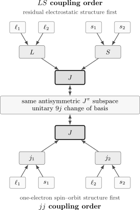
LS and jj coupling pair the same one-electron angular momenta in different orders. Properly antisymmetrized bases end in the same $J^\pi$ subspace and are related by a unitary recoupling transformation; the Hamiltonian hierarchy determines which basis is economical.

The Hamiltonian Hierarchy

A useful schematic partition for a multi-electron atom is

$$H=H_{\mathrm{cf+so}}+V_{\mathrm{res}}+H_{\mathrm{small}},$$

where

• $H_{\mathrm{cf+so}}$ is a sum of one-electron central-field Hamiltonians with spin–orbit or Dirac structure already included;
• $V_{\mathrm{res}}$ contains the residual electron–electron interaction not absorbed into the central field;
• $H_{\mathrm{small}}$ collects additional Breit, recoil, radiative, nuclear, and external-field terms at the required accuracy.

In a nonrelativistic reduction, the first part may be represented as

$$H_{\mathrm{cf+so}} = \sum_i \left[ h_{\mathrm{cf}}(i) + \zeta_i\, \frac{\mathbf l_i\cdot\mathbf s_i}{\hbar^2} \right].$$

In a relativistic calculation, one instead starts from central-field Dirac spinors, so spin–orbit structure is not appended as a separate perturbation. The labels $n\kappa jm_j$ then arise directly from the one-electron eigenproblem.

The jj limit is useful when the separations among relevant $n\ell_j$ subshells are large compared with the residual off-diagonal matrix elements that change those occupations or parent couplings. For two jj-coupled configuration-state functions of the same exact $J$ and parity,

$$|aJM\pi\rangle, \qquad |bJM\pi\rangle,$$

a local mixing estimate is

$$\epsilon_{ab} = \frac{ \left| \langle bJM\pi| V_{\mathrm{res}} |aJM\pi\rangle \right| }{ \left| E_a^{(0)}-E_b^{(0)} \right| }.$$

If $\epsilon_{ab}\ll1$ for all nearby competitors that matter to an observable, the corresponding jj labels are stable. If a denominator becomes small, one pair of levels can mix strongly even when most of the spectrum remains close to jj coupling. There is therefore no universal atomic number at which jj coupling “turns on.”

Exact and approximate labels

For an isolated, field-free atom with a rotationally invariant and parity-conserving electronic Hamiltonian,

$$[H,J^2]=[H,J_z]=[H,\mathcal P]=0.$$

Total $J$, its projection $M$, and parity $\pi$ can be exact. By contrast, residual interactions generally imply

$$[H,j_i^2]\neq0$$

for an individually named electron, and they can also mix configuration-state functions with different relativistic-subshell occupations. The $j_i$, subshell-parent $J_r$, and occupation labels are therefore approximate unless the chosen Hamiltonian makes them exact.

This distinction matters because electrons are indistinguishable. A phrase such as “electron 1 has $j_1=1/2$” is construction language in a labeled-particle derivation. An antisymmetric atomic state is more faithfully described by occupations of one-electron spinors and by coupled subshell parents.

Individual-Electron j

For electron spin $s=1/2$, adding orbital angular momentum $\ell$ gives

$$j= \begin{cases} \ell+\dfrac12,\\[4pt] \ell-\dfrac12, & \ell>0. \end{cases}$$

The coupled angular-spin state is

$$\begin{aligned} |\ell,\tfrac12;jm\rangle ={}& \sum_{m_\ell,m_s} \langle \ell m_\ell,\tfrac12 m_s \vert jm \rangle\\ &\times |\ell m_\ell\rangle |\tfrac12 m_s\rangle. \end{aligned}$$

In coordinate space this coupling is packaged by a spinor spherical harmonic. The detailed functions and phase conventions are developed in Addition of Orbital and Spin Angular Momentum; jj coupling uses them as one-electron building blocks.

Dirac angular label

Relativistic central-field calculations commonly replace the pair $(\ell,j)$ by the nonzero integer

$$\kappa= \begin{cases} -(\ell+1), &j=\ell+\dfrac12,\\[5pt] +\ell, &j=\ell-\dfrac12. \end{cases}$$

Equivalently,

$$\kappa = (-1)^{j+\ell+1/2} \left(j+\frac12\right).$$

The labels $j$ and $\kappa$ do not have the same content: $j=1/2$ can describe either $s_{1/2}$ or $p_{1/2}$, whereas the sign and magnitude of $\kappa$ distinguish their orbital and parity structure. The parity of a one-electron spinor remains

$$\pi=(-1)^\ell.$$

For formula-level relativistic context, see the Dirac Equation. A many-electron jj label does not by itself assert that a particular no-pair Dirac–Coulomb, Breit, or QED Hamiltonian was used; the calculation must state that separately.

Spin–orbit eigenvalues

The identity

$$2\mathbf l\cdot\mathbf s = j^2-l^2-s^2$$

gives

$$\frac{ \langle\mathbf l\cdot\mathbf s\rangle }{\hbar^2} = \frac12 \left[ j(j+1)-\ell(\ell+1)-\frac34 \right].$$

For the two branches,

$$\frac{ \langle\mathbf l\cdot\mathbf s\rangle }{\hbar^2} = \begin{cases} \dfrac{\ell}{2}, &j=\ell+\dfrac12,\\[6pt] -\dfrac{\ell+1}{2}, &j=\ell-\dfrac12. \end{cases}$$

With the convention

$$H_{\mathrm{so}} = \zeta\, \frac{\mathbf l\cdot\mathbf s}{\hbar^2},$$

the separation of the two branches is

$$E_{\ell+1/2}-E_{\ell-1/2} = \frac{2\ell+1}{2}\,\zeta.$$

This is an angular result for an effective one-electron spin–orbit model. The sign and magnitude of $\zeta$, radial relaxation, two-electron fine-structure terms, and fully relativistic effects belong to the declared atomic Hamiltonian.

Relativistic-subshell capacity

A fixed $n\ell_j$ subshell contains

$$2j+1$$

magnetic spinors. Thus

nonrelativistic subshell	relativistic subshells	capacities
$s$	$s_{1/2}$	$2$
$p$	$p_{1/2}$, $p_{3/2}$	$2$, $4$
$d$	$d_{3/2}$, $d_{5/2}$	$4$, $6$
$f$	$f_{5/2}$, $f_{7/2}$	$6$, $8$

The totals remain $2(2\ell+1)$. Splitting a nonrelativistic subshell changes the basis and energy organization, not the number of one-electron modes.

Building jj-Coupled Atomic States

Two non-equivalent electrons

For two non-equivalent one-electron angular momenta, the coupled basis is

$$\begin{aligned} |(j_1j_2)JM\rangle = \sum_{m_1,m_2} &\langle j_1m_1,j_2m_2 \vert JM \rangle\\ &\times |j_1m_1\rangle |j_2m_2\rangle. \end{aligned}$$

The allowed totals are

$$J= |j_1-j_2|, |j_1-j_2|+1, \ldots, j_1+j_2.$$

The dimension check is

$$(2j_1+1)(2j_2+1) = \sum_{J=|j_1-j_2|}^{j_1+j_2}(2J+1).$$

When the one-electron orbitals differ, the full electronic state must still be antisymmetrized. “Non-equivalent” means the orbitals carry different radial or angular labels; it does not make the electrons distinguishable.

Subshell parents and sequential coupling

For several open relativistic subshells, first couple the electrons within each subshell to a parent angular momentum $J_r$, then couple the parents. A schematic two-subshell configuration-state function is

$$\left| \left[ (n_1\ell_1j_1)^{q_1}\alpha_1J_1, (n_2\ell_2j_2)^{q_2}\alpha_2J_2 \right] JM\pi \right\rangle.$$

The labels $\alpha_r$ distinguish repeated states with the same subshell occupation and parent $J_r$. They can encode seniority, quasispin, or an additional parentage convention. For more subshells, parentheses or an explicit coupling tree are essential because intermediate angular momenta depend on the order of addition.

Compact spectroscopic labels often suppress radial labels, closed subshells, intermediate parents, or $M$. For example,

$$(6p_{1/2}^{\,2})_0$$

means that the two electrons occupy the $6p_{1/2}$ relativistic subshell and form parent $J=0$. A compact label should not be read as a complete wavefunction.

Configuration-state functions

A jj-coupled configuration-state function is an antisymmetric eigenfunction of $J^2$, $J_z$, and parity constructed from one-electron spinors. In a determinant basis,

$$|\Gamma JM\pi\rangle = \sum_I c_I^{(\Gamma J\pi)} |\Phi_I\rangle,$$

where every determinant in the sum has the same total projection $M$ and parity, while the coefficients project onto definite total $J$ and the declared parent labels.

An exact or approximate atomic eigenstate is then another expansion,

$$|\Psi_{\nu JM\pi}\rangle = \sum_\Gamma C_{\Gamma}^{(\nu J\pi)} |\Gamma JM\pi\rangle.$$

The first transformation builds symmetry-adapted basis states. The second diagonalizes the Hamiltonian. Confusing these two steps makes a basis label look more exact than it is.

Equivalent Electrons and Pauli Restrictions

Two electrons in the same $n\ell_j$ subshell cannot realize every total $J$ allowed by the ordinary triangle rule. Before antisymmetrization, interchange of the two equal-$j$ angular factors gives

$$P_{12}|(jj)JM\rangle = (-1)^{2j-J}|(jj)JM\rangle.$$

Electrons require exchange eigenvalue $-1$. Since electronic $j$ is half-integer, $2j$ is odd, so a pair in the same radial and angular spinor subshell permits

$$J=0,2,4,\ldots,2j-1.$$

Examples are

$$\begin{array}{ccl} (p_{1/2}^{\,2})&:&J=0,\\ (p_{3/2}^{\,2})&:&J=0,2,\\ (d_{5/2}^{\,2})&:&J=0,2,4. \end{array}$$

The corresponding state count for $j=5/2$ is

$$1+5+9=15 = \binom{2j+1}{2}.$$

This equality is a useful check that antisymmetry has neither omitted nor duplicated states. For three or more equivalent electrons, total $J$ may occur more than once. Seniority and coefficients of fractional parentage then organize the allowed subshell states; listing the triangle-rule values of $J$ is not enough.

Worked Example: The p² Configuration

A nonrelativistic $p$ subshell has six spin-orbitals, so two electrons span

$$\binom62=15$$

antisymmetric states. In a jj basis, distribute the electrons between the $p_{1/2}$ and $p_{3/2}$ subshells.

jj sector	allowed parent $J$	magnetic-state count
$(p_{1/2}^{\,2})_0$	$0$	$1$
$(p_{1/2}p_{3/2})_J$	$1,2$	$3+5=8$
$(p_{3/2}^{\,2})_J$	$0,2$	$1+5=6$

Therefore

$$1+8+6=15,$$

as required.

The same configuration in an $LS$ basis has the allowed terms

$${}^1S_0, \qquad {}^1D_2, \qquad {}^3P_{0,1,2}.$$

Their dimensions also give

$$1+5+(1+3+5)=15.$$

The fixed-$J$ comparison is especially informative:

exact $J$ sector	LS basis	jj basis
$0$	$\,{}^1S_0$, $\,{}^3P_0$	$(p_{1/2}^{\,2})_0$, $(p_{3/2}^{\,2})_0$
$1$	$\,{}^3P_1$	$(p_{1/2}p_{3/2})_1$
$2$	$\,{}^1D_2$, $\,{}^3P_2$	$(p_{1/2}p_{3/2})_2$, $(p_{3/2}^{\,2})_2$

Within the complete $p^2$ configuration, the $J=1$ sector contains only one multiplet. Its normalized LS and jj basis vectors must therefore agree up to phase. The $J=0$ and $J=2$ sectors are two-dimensional, so each coupling scheme supplies a different orthonormal pair. The Hamiltonian decides which linear combinations approximate the observed levels.

This example prevents a common misconception: jj coupling does not create additional levels. It reorganizes the same antisymmetric state space around relativistic-subshell occupations.

Comparison with LS Coupling

For two electrons, the two limiting coupling orders are

$$\begin{aligned} LS:\quad &(\mathbf l_1+\mathbf l_2)=\mathbf L, \qquad (\mathbf s_1+\mathbf s_2)=\mathbf S,\\ &\mathbf L+\mathbf S=\mathbf J, \end{aligned}$$

and

$$\begin{aligned} jj:\quad &(\mathbf l_1+\mathbf s_1)=\mathbf j_1, \qquad (\mathbf l_2+\mathbf s_2)=\mathbf j_2,\\ &\mathbf j_1+\mathbf j_2=\mathbf J. \end{aligned}$$

Both constructions diagonalize the same exact total $J^2$ and $J_z$. Their intermediate operators differ. In ideal LS coupling, $L^2$ and $S^2$ are approximately diagonal in the Hamiltonian. In ideal jj coupling, one-electron $j_i^2$ values and relativistic-subshell occupations are approximately stable.

• Dominant organization: LS coupling follows residual electrostatic terms; jj coupling follows one-electron spin–orbit or relativistic-subshell splitting.
• First coupling step: LS combines all $\mathbf l_i$ into $\mathbf L$ and all $\mathbf s_i$ into $\mathbf S$; jj combines each $\mathbf l_i+\mathbf s_i$ into $\mathbf j_i$.
• Natural labels: LS uses $\gamma\,{}^{2S+1}L_J^\pi$; jj uses relativistic occupations, subshell parents, and final $J^\pi$.
• Exact field-free labels: both schemes retain total $J$, $M$, and parity when the Hamiltonian has the corresponding symmetries.
• Approximate labels: $L$, $S$, and configuration can mix in LS language; $j$ occupations, parent $J_r$, and configuration can mix in jj language.
• Characteristic failure: each limiting description fails through off-diagonal mixing among configuration-state functions with the same exact $J^\pi$.

The words “weak” and “strong” spin–orbit coupling must refer to a comparison. A spin–orbit splitting of fixed numerical size can be weak relative to broad electrostatic term separations but strong relative to a nearby same-$J^\pi$ separation.

The one-open-electron caution

For a closed core plus one open electron, the labels

$${}^2L_J \qquad\text{and}\qquad n\ell_j$$

describe the same angular coupling because $L=\ell$, $S=1/2$, and $J=j$. A resolved $p_{1/2}$–$p_{3/2}$ doublet is evidence for one-electron spin–orbit structure, but it does not by itself diagnose a nontrivial many-electron jj coupling regime. The distinction becomes substantive when two or more open angular momenta admit competing coupling orders.

LS-to-jj Recoupling

For two labeled electrons, define the abbreviated basis states

$$\begin{aligned} |jj;JM\rangle &\equiv |[(\ell_1s_1)j_1,(\ell_2s_2)j_2]JM\rangle,\\ |LS;JM\rangle &\equiv |[(\ell_1\ell_2)L,(s_1s_2)S]JM\rangle. \end{aligned}$$

Under the standard Condon–Shortley angular-momentum convention, write their overlap as

$$\begin{aligned} \mathcal U^J_{LS,j_1j_2} &\equiv \langle jj;JM|LS;JM\rangle\\ &= \widehat L\, \widehat S\, \widehat j_1\, \widehat j_2\\ &\quad\times \left\{ \begin{array}{ccc} \ell_1&s_1&j_1\\ \ell_2&s_2&j_2\\ L&S&J \end{array} \right\}. \end{aligned}$$

where

$$\widehat x\equiv\sqrt{2x+1}.$$

The braces contain a Wigner $9j$ symbol. The coefficient is independent of $M$ because both bases transform as the same total-$J$ irreducible representation. Different state-ordering and phase conventions can change row or column signs, but not level energies, probabilities, or transition strengths calculated consistently.

For equivalent electrons, the labeled-particle formula must be restricted to properly normalized antisymmetric states. Once forbidden sectors are removed and repeated states are resolved, the resulting LS-to-jj matrix is unitary:

$$\sum_{LS} \mathcal U^J_{LS,\beta} \mathcal U^{J*}_{LS,\beta'} = \delta_{\beta\beta'}.$$

Here $\beta$ denotes the allowed jj occupation and parent labels in the fixed-$J$ sector. Unitarity is the precise statement that recoupling changes coordinates, not physical states.

What a recoupling coefficient does not tell you

A $9j$ coefficient answers how two basis choices overlap. It does not determine which basis diagonalizes the atomic Hamiltonian. That requires radial integrals, electron–electron matrix elements, relativistic terms, and often configuration interaction. Angular algebra supplies the allowed structure; dynamics supplies the eigenvectors and energies.

Intermediate Coupling

Most real open-shell spectra are neither pure LS nor pure jj. The disciplined treatment is to diagonalize the chosen Hamiltonian inside every exact symmetry block:

$$\sum_b H^{J\pi}_{ab}C_b^{(\nu)} = E_{\nu J\pi}C_a^{(\nu)}.$$

The eigenstate may be expanded in either basis,

$$\begin{aligned} |\Psi_{\nu J\pi}\rangle &= \sum_\alpha A_\alpha^{(\nu)} |\alpha LSJ\pi\rangle\\ &= \sum_\beta B_\beta^{(\nu)} |\beta jj;J\pi\rangle. \end{aligned}$$

The coefficients are related by the unitary recoupling matrix. Neither expansion is more physical in the abstract; one may be more compact and more interpretable for the Hamiltonian and observable under study.

Purity must name a basis

A statement such as “the level is 82% jj coupled” is incomplete unless it specifies:

• the orbital set and configuration space;
• the jj configuration-state function or grouped subspace;
• the Hamiltonian and calculation;
• whether the percentage is one coefficient squared or a sum over several components.

For an orthonormal jj basis, the weight of a declared subspace $\mathcal B$ is

$$w_{\mathcal B}^{(jj)} = \sum_{\beta\in\mathcal B} |B_\beta|^2.$$

The analogous LS weight uses the $A_\alpha$. Individual coefficients can change under unitary rotations among basis functions carrying the same displayed labels. A projector onto a fully declared subspace is more robust than a single unnamed “percentage.”

Two-level model

When two same-$J^\pi$ basis states dominate, write

$$H= \begin{pmatrix} E_a&V\\ V^*&E_b \end{pmatrix}.$$

After choosing phases so that the relevant coupling is real, the mixing angle satisfies

$$|\tan(2\theta)| = \frac{2|V|}{|E_a-E_b|}.$$

Far from a crossing, $|V|\ll|E_a-E_b|$ gives a small minority amplitude. Near an avoided crossing, even a modest $V$ can produce nearly equal mixtures. Along an isoelectronic sequence, labels should therefore be tracked by eigenvector overlaps and observables, not by energy order alone.

Intermediate coupling is not a thermodynamic phase transition. It is a statement that no single limiting coupling basis makes every relevant eigenvector nearly pure.

Spectroscopic Diagnostics

No single datum proves jj coupling. A reliable assignment combines energy patterns, calculated eigenvectors, magnetic response, and transitions.

Energy clustering

In a strong jj limit, the gross separation between configurations that differ in $n\ell_{\ell-1/2}$ and $n\ell_{\ell+1/2}$ occupations reflects the one-electron relativistic-subshell separation. Residual electrostatic interactions then split the allowed parent-$J$ levels within each occupation pattern.

This order reverses the ideal LS narrative, where electrostatic terms form first and spin–orbit interactions split each term into $J$ levels. Real spectra can contain both kinds of spacing, and accidental near-degeneracies can obscure either pattern.

Eigenvector composition

Atomic-structure calculations often report leading percentages. These are useful when the basis, normalization, and omitted remainder are stated. The NIST Atomic Spectra Database may display leading components in LS, jj, or another coupling convention, reflecting whichever description makes a level assignment most informative.

A level name is not an observable. If two calculated components are comparable, reporting both is more trustworthy than forcing a pure label. Assignments can also change as the configuration-interaction expansion or Hamiltonian is improved.

Magnetic factors

For one electron with orbital and spin magnetic factors $g_L$ and $g_S$, projection onto $\mathbf j=\mathbf l+\mathbf s$ gives

$$\begin{aligned} g_j &= g_L+(g_S-g_L)Q_j,\\ Q_j &= \frac{ j(j+1)+s(s+1)-\ell(\ell+1) }{ 2j(j+1) }. \end{aligned}$$

For two approximately independent angular momenta $\mathbf j_1$ and $\mathbf j_2$ coupled to nonzero $J$, define

$$\begin{aligned} C_1&= \frac{ J(J+1)+j_1(j_1+1)-j_2(j_2+1) }{ 2J(J+1) },\\ C_2&= \frac{ J(J+1)-j_1(j_1+1)+j_2(j_2+1) }{ 2J(J+1) }. \end{aligned}$$

Then the ideal jj-coupled factor is

$$g_J=g_{j_1}C_1+g_{j_2}C_2.$$

This projection formula generalizes recursively to coupled subshell parents. It is a diagnostic, not an exact many-electron theorem: configuration mixing, relativistic magnetic operators, core polarization, QED corrections, and nuclear coupling can shift measured factors. For $J=0$, the formula is undefined and there is no ordinary first-order electronic Zeeman splitting proportional to $M$.

Transition patterns

For an electric-dipole transition in an isolated parity eigenstate, the robust electronic constraints are

$$\begin{aligned} \pi_f&=-\pi_i,\\ \Delta J&=0,\pm1,\\ J_i=J_f=0 &\quad\text{forbidden}. \end{aligned}$$

Rules involving a particular $j$ occupation, subshell parent, or spectator electron are limiting-basis statements. A one-body electric-dipole operator often makes them useful in a pure jj description, with $6j$ symbols carrying the recoupling factors, but configuration and intermediate-coupling admixtures can open nominally forbidden branches.

Transition amplitudes can be more sensitive to small admixtures than energies. A component with only a few percent probability can dominate a line if the leading component has a vanishing matrix element. The full operator treatment belongs to Atomic Selection Rules and Applications to Atomic Spectra.

Spectroscopic Examples

Heavy 6p ground configurations

The NIST atomic-spectroscopy compendium identifies the large $6p$ spin–orbit interaction as producing useful jj structures for the ground configurations of neutral lead, bismuth, and polonium. Compact leading labels are

$$\begin{aligned} \mathrm{Pb\,I}:&\quad (6p_{1/2}^{\,2})_0,\\ \mathrm{Bi\,I}:&\quad (6p_{1/2}^{\,2}6p_{3/2})^\circ_{3/2},\\ \mathrm{Po\,I}:&\quad (6p_{1/2}^{\,2}6p_{3/2}^{\,2})_2. \end{aligned}$$

The superscript circle marks odd parity for the $6p^3$ bismuth configuration. The closed $6p_{1/2}^{\,2}$ pair has parent $J=0$, so the remaining $6p_{3/2}$ electron gives Bi I total $J=3/2$. In Po I, two $6p_{3/2}$ electrons may couple to $J=0$ or $2$; the displayed label identifies the ground level as the $J=2$ parent.

These labels summarize dominant angular structure. They do not assert 100% purity, omit all configuration interaction, or replace evaluated energies and eigenvector compositions. The associated NIST data record and calculation should be consulted whenever a quantitative assignment matters.

Particle–hole shorthand

Near a filled relativistic subshell, hole notation can shorten a label. A subshell of capacity $2j+1$ with $q$ electrons may equivalently be described by

$$q_{\mathrm h}=2j+1-q$$

holes. A hole carries the same angular-momentum magnitude $j$, but magnetic moments, phases, parentage, and energy conventions require care. Negative occupation exponents sometimes used in tabulations are notation, not negative particle numbers.

A spectrum-wide diagnosis

Suppose a heavy-atom calculation finds:

1. level groups separated mainly by $p_{1/2}$ versus $p_{3/2}$ occupation;
2. leading jj weights of $80$–$95\%$ for most levels;
3. measured $g$ factors close to jj projections;
4. line strengths broadly following the same parentage pattern.

It is then reasonable to call the spectrum predominantly jj coupled, while naming strongly mixed exceptions. If only the energy grouping agrees but eigenvectors and magnetic factors do not, the assignment remains provisional.

Common Mistakes

• Treating jj coupling as a different Hilbert space. Complete LS and jj bases span the same fixed-configuration state space.
• Using atomic number as the criterion. The relevant ratios are local off-diagonal matrix elements divided by nearby same-$J^\pi$ separations.
• Calling every relativistic calculation pure jj coupling. Relativistic spinors provide a jj-oriented basis, but the correlated eigenvectors can still be strongly mixed.
• Applying the triangle rule to equivalent electrons without Pauli restrictions. A pair in one half-integer-$j$ subshell permits only even $J$.
• Assigning persistent labels to individual electrons. Atomic states are antisymmetric; relativistic-subshell occupations and parent couplings are the appropriate many-electron language.
• Omitting coupling parentheses. For several open subshells, intermediate parent angular momenta depend on the declared coupling tree.
• Interpreting a leading percentage as an observable. It depends on the orbital set, configuration space, and basis convention.
• Diagnosing many-electron jj coupling from a one-electron doublet. Closed-core plus one-electron LS and jj labels are equivalent.
• Assuming energy agreement proves wavefunction quality. Magnetic factors and line strengths test different projections of the eigenvector.
• Using pure-coupling transition rules as exact symmetries. Total $J$ and parity rules are more robust than subshell-parent selection rules.

Exercises

Exercise 1: A d-electron spin–orbit pair

For $\ell=2$ and $s=1/2$, find the two $j$ values, their capacities, the eigenvalues of $\mathbf l\cdot\mathbf s/\hbar^2$, and their separation for

$$H_{\mathrm{so}} = \zeta\, \frac{\mathbf l\cdot\mathbf s}{\hbar^2}.$$

Solution

The allowed angular momenta are

$$j=\frac52 \qquad\text{and}\qquad j=\frac32.$$

Their capacities are

$$2j+1=6 \qquad\text{and}\qquad 2j+1=4,$$

which sum to the ten spin-orbitals of a nonrelativistic $d$ subshell. The angular eigenvalues are

$$\begin{aligned} j=\frac52:\quad &\frac{ \langle\mathbf l\cdot\mathbf s\rangle }{\hbar^2} =\frac{\ell}{2}=1,\\ j=\frac32:\quad &\frac{ \langle\mathbf l\cdot\mathbf s\rangle }{\hbar^2} =-\frac{\ell+1}{2}=-\frac32. \end{aligned}$$

Therefore

$$E_{5/2}-E_{3/2} = \left(1+\frac32\right)\zeta = \frac52\zeta.$$

The sign of $\zeta$ determines which branch lies higher in this effective model.

Exercise 2: Couple two non-equivalent j values

Two non-equivalent open electrons have $j_1=1/2$ and $j_2=3/2$. List the allowed total $J$ values and verify the product-space dimension.

Solution

The triangle rule gives

$$J= \left|\frac12-\frac32\right|, \ldots, \frac12+\frac32,$$

so

$$J=1,2.$$

Their magnetic dimensions are $3$ and $5$, hence

$$3+5=8.$$

The uncoupled product has dimension

$$(2j_1+1)(2j_2+1) = 2\cdot4=8.$$

The equality confirms that both allowed multiplets appear once.

Exercise 3: Equivalent electrons in a j = 5/2 subshell

Use the exchange phase to find the allowed $J$ values for two equivalent electrons in a $j=5/2$ subshell. Check the result against the number of determinant occupations.

Solution

Interchange gives the phase

$$(-1)^{2j-J}=(-1)^{5-J}.$$

Fermionic antisymmetry requires this phase to be $-1$, so $J$ must be even. The triangle rule allows $J=0,1,\ldots,5$, and the surviving values are

$$J=0,2,4.$$

Their total number of magnetic states is

$$\begin{aligned} &(2\cdot0+1) +(2\cdot2+1) +(2\cdot4+1)\\ &\qquad=1+5+9=15. \end{aligned}$$

The subshell contains six magnetic spinors, so direct occupation counting gives

$$\binom62=15.$$

The two counts agree.

Exercise 4: Recount p² in both coupling schemes

List the allowed jj sectors of $p^2$, count their magnetic states, and compare with the LS terms. Which fixed-$J$ sector has no nontrivial recoupling freedom?

Solution

The allowed jj sectors are

$$\begin{aligned} (p_{1/2}^{\,2})&:\quad J=0,\\ (p_{1/2}p_{3/2})&:\quad J=1,2,\\ (p_{3/2}^{\,2})&:\quad J=0,2. \end{aligned}$$

Their state count is

$$1+(3+5)+(1+5)=15.$$

The LS terms are

$${}^1S_0,\qquad{}^1D_2,\qquad{}^3P_{0,1,2},$$

with count

$$1+5+(1+3+5)=15.$$

Only one $J=1$ multiplet occurs in either description. Therefore the normalized $\,{}^3P_1$ and $(p_{1/2}p_{3/2})_1$ states agree up to phase within the complete $p^2$ configuration. The $J=0$ and $J=2$ sectors each contain two multiplets and support nontrivial $2\times2$ recoupling matrices.

Exercise 5: Why the 9j overlap is independent of M

Explain why the LS-to-jj recoupling coefficient for fixed $J$ cannot depend on the magnetic quantum number $M$. What role does the $9j$ matrix play when a Hamiltonian is represented in the two bases?

Solution

Both basis states are magnetic components of the same total-$J$ irreducible representation. A change in coupling order acts on the multiplicity labels that distinguish copies of that representation; it does not select an orientation in space. Rotational covariance therefore makes the overlap independent of $M$.

In a complete fixed-$J^\pi$ space, the $9j$ coefficients assemble into a unitary matrix $\mathcal U$. If $H_{LS}$ is the Hamiltonian matrix in the LS basis, then the jj representation is

$$H_{jj} = \mathcal U^\dagger H_{LS} \mathcal U.$$

The matrices have identical eigenvalues. A basis may make one matrix closer to diagonal, but a unitary recoupling does not alter the exact spectrum.

Exercise 6: Magnetic factors for p₁/₂ and p₃/₂

Set $g_L=1$ and $g_S=2$. Find the one-electron factors for $p_{1/2}$ and $p_{3/2}$. Then couple one electron of each type and find the ideal jj factors for $J=1$ and $J=2$.

Solution

For $\ell=1$ and $s=1/2$, the one-electron Landé formula gives

$$g_{p_{1/2}}=\frac23, \qquad g_{p_{3/2}}=\frac43.$$

For $j_1=1/2$, $j_2=3/2$, and $J=1$,

$$C_1=-\frac14, \qquad C_2=\frac54.$$

Hence

$$g_{J=1} = \frac23\left(-\frac14\right) + \frac43\left(\frac54\right) = \frac32.$$

For $J=2$,

$$C_1=\frac14, \qquad C_2=\frac34,$$

so

$$g_{J=2} = \frac23\left(\frac14\right) + \frac43\left(\frac34\right) = \frac76.$$

These are limiting-basis predictions. Configuration mixing and corrections to the magnetic operator can move the measured values.

Exercise 7: Diagnose a mixed heavy-atom level

A calculation in a declared orbital and configuration space gives a level with $82\%$ weight in one jj parent subspace but only $55\%$ weight in its leading LS term. Nearby energies cluster according to relativistic-subshell occupation, and the measured $g$ factor agrees with the jj estimate within $3\%$. What conclusion is justified, and what would be an overclaim?

Solution

The larger jj weight, occupation-based energy clustering, and magnetic agreement jointly support a predominantly jj-coupled assignment. The remaining $18\%$ outside the leading jj subspace is nevertheless substantial, so the level belongs to intermediate coupling rather than an exact jj limit.

A defensible description is: “The level is predominantly described by the stated jj parent, with measurable intermediate-coupling admixture in the declared calculation.” It would be an overclaim to call the $j$ occupations exact, to infer that every transition obeys pure-jj parentage rules, or to quote the $82\%$ without naming the basis and model space.

The $55\%$ LS weight is not inconsistent with the jj assignment. LS and jj percentages refer to different projectors after a unitary change of basis.

Key Takeaways

• jj coupling first combines each $\mathbf l_i$ with $\mathbf s_i$, then couples the resulting $\mathbf j_i$ or subshell parents to total $\mathbf J$.
• It is a useful physical limit when relativistic-subshell separations dominate residual same-$J^\pi$ mixing; “heavy atom” is only a clue.
• Total $J$ and parity can be exact while individual $j$ occupations and parent angular momenta remain approximate.
• Equivalent electrons require Pauli restrictions beyond the triangle rule; two electrons in one half-integer-$j$ subshell allow even $J$ only.
• Complete LS and jj bases contain the same states and are related by unitary $9j$ recoupling.
• The $p^2$ configuration has 15 antisymmetric states in either basis; only its $J=0$ and $J=2$ sectors have nontrivial LS-to-jj mixing.
• Intermediate-coupling percentages are meaningful only after the basis, orbital set, and grouped subspace are declared.
• Energies, eigenvectors, magnetic factors, and line strengths provide complementary coupling diagnostics.
• Exact E1 constraints are best stated through total $J$ and parity; jj parentage rules are limiting-basis statements.

Cross-Links

• Term Symbol Reference compares jj group labels with LS and molecular symbol grammars.
• Multi-Electron Atoms
• Electron Configurations
• Pauli Principle in Atoms
• Slater Determinants in Atoms
• LS Coupling
• Hund’s Rules
• Atomic Term Symbols
• Fine Structure
• Atomic Selection Rules
• Zeeman Effect in Atoms
• Angular Momentum Coupling Schemes
• Addition of Orbital and Spin Angular Momentum
• Spin–Orbit Coupling
• Recoupling and Wigner Symbols
• Applications to Atomic Spectra
• Dirac Equation
• AMO Physics Roadmap

References

1. W. C. Martin and W. L. Wiese, “Atomic Spectroscopy: An Introduction”, in G. W. F. Drake, ed., Atomic, Molecular, and Optical Physics Handbook, AIP Press, 1996; NIST online revision updated 2025.
2. W. C. Martin and W. L. Wiese, “Allowed Terms”, NIST Atomic Spectroscopy Compendium, updated 2025.
3. W. C. Martin and W. L. Wiese, “Different Coupling Schemes”, NIST Atomic Spectroscopy Compendium, updated 2025.
4. W. C. Martin and W. L. Wiese, “Eigenvector Composition of Levels”, NIST Atomic Spectroscopy Compendium, updated 2025.
5. A. Kramida, Yu. Ralchenko, J. Reader, and the NIST ASD Team, NIST Atomic Spectra Database, version 5.12, National Institute of Standards and Technology, 2024, DOI: 10.18434/T4W30F, accessed 2026-07-21.
6. E. U. Condon and G. H. Shortley, The Theory of Atomic Spectra, Cambridge University Press, 1935.
7. R. D. Cowan, The Theory of Atomic Structure and Spectra, University of California Press, 1981.
8. I. P. Grant, Relativistic Quantum Theory of Atoms and Molecules: Theory and Computation, Springer, 2007.
9. W. R. Johnson, Atomic Structure Theory: Lectures on Atomic Physics, Springer, 2007.
10. I. I. Sobelman, Atomic Spectra and Radiative Transitions, 2nd ed., Springer, 1992.
11. R. N. Zare, Angular Momentum: Understanding Spatial Aspects in Chemistry and Physics, Wiley, 1988.
12. C. Froese Fischer, T. Brage, and P. Jönsson, Computational Atomic Structure: An MCHF Approach, Institute of Physics Publishing, 1997.
13. B. R. Judd, Operator Techniques in Atomic Spectroscopy, McGraw–Hill, 1963.