Pauli Principle in Atoms

The Pauli principle in an atom is not merely a rule for drawing arrows in orbital boxes. It is the requirement that the total state of the identical electrons be antisymmetric under exchange of any two complete electron coordinates. The familiar statement that no two electrons can have the same four atomic quantum numbers is a basis-dependent consequence of that deeper rule.

Antisymmetry is indispensable for shell capacities, closed subshells, equivalent-electron term restrictions, and the recurring valence patterns behind chemistry. It does not by itself determine orbital energies, the order in which subshells fill, or the energy ordering of allowed terms. Those require the atomic Hamiltonian.

A careful summary is:

The one-electron spectrum supplies the available modes; fermionic antisymmetry restricts how electrons may occupy and combine them; interactions determine the energies of the allowed states.

Canonical Scope

This page owns the atomic consequences of the Pauli principle: complete spin-orbitals, subshell capacities, atomic determinants, equivalent-electron restrictions, closed-shell structure, and the qualified connection to periodicity.

Several neighboring pages own the underlying or downstream subjects:

• Pauli Exclusion Principle gives the general derivation from fermionic antisymmetry.
• Spin and Spatial Wavefunctions develops the singlet–triplet exchange pairing.
• Slater Determinants develops determinant algebra and normalization.
• Slater Determinants in Atoms applies that algebra to atomic projection sectors, configurations, and configuration-state functions.
• Electron Configurations owns subshell notation, Aufbau reasoning, and configuration mixing.
• Atomic Term Symbols owns the grammar of terms and fine-structure levels.
• Pauli Exclusion Principle: Historical Context follows the route from spectroscopy to Pauli’s 1925 rule.

Here those ideas are applied to the structure of actual atomic state spaces without rederiving their full general theory.

The Exact Atomic Statement

Let

$$x_i=(\mathbf r_i,\sigma_i)$$

denote the spatial and spin coordinates in electron slot $i$. For every transposition $P_{ij}$, a physical $N$-electron state obeys

$$P_{ij}\Psi(x_1,\ldots,x_N) =-\Psi(x_1,\ldots,x_N).$$

More generally,

$$P_{\pi}\Psi =\operatorname{sgn}(\pi)\Psi$$

for every permutation $\pi\in S_N$. The physical fixed-$N$ Hilbert space is the antisymmetric exterior power

$$\mathcal H_N^{(\mathrm e)} =\bigwedge^N\mathcal h,$$

where $\mathcal h$ is the complete one-electron Hilbert space.

Electron labels in $\Psi(x_1,\ldots,x_N)$ identify argument slots, not persistent particles. Exchanging slots changes the amplitude’s sign, while all probabilities and expectation values remain permutation invariant.

Exclusion is not a potential

The Pauli principle does not add a repulsive term to the Hamiltonian. It restricts the admissible state space before the Coulomb Hamiltonian is diagonalized. Phrases such as “Pauli repulsion” or “exchange force” can summarize an energy cost caused by antisymmetry and orbital overlap, but they should not be mistaken for a new pair potential.

This distinction becomes important when separating exchange from dynamical electron correlation. Both affect spatial avoidance and energies, but they enter the theory in different ways.

Complete One-Electron Spin-Orbitals

In a nonrelativistic central field, a one-electron spatial orbital has labels $n,\ell,m_\ell$. Combining it with a spin basis gives

$$\begin{aligned} \chi_{n\ell m_\ell m_s}(x) &=\phi_{n\ell m_\ell}(\mathbf r)\\ &\quad\times\omega_{m_s}(\sigma),\\ m_s&=\pm\frac12. \end{aligned}$$

The complete one-electron mode includes the spin label. Thus

$$\phi_a(\mathbf r)\alpha(\sigma) \quad\text{and}\quad \phi_a(\mathbf r)\beta(\sigma)$$

are distinct spin-orbitals even though they share the same spatial orbital.

For a fixed $n\ell$ subshell, there are

$$(2\ell+1)\times2 =2(2\ell+1)$$

spin-orbitals. Pauli exclusion permits at most one electron in each complete spin-orbital, so the subshell capacities are $2$, $6$, $10$, and $14$ for $s$, $p$, $d$, and $f$.

Relativistic basis

In a relativistic central field, a spinor may instead be labeled by $n,\kappa,j,m_j$ or $n\ell_jm_j$. A fixed-$j$ subshell has $2j+1$ modes, each with occupation zero or one. The Pauli principle is basis independent; only the labels used to enumerate the one-electron modes have changed.

Three Equivalent Forms of Exclusion

The same atomic restriction appears in coordinate, determinant, and operator language.

Antisymmetric pair

For two spin-orbitals $\chi_a$ and $\chi_b$,

$$\begin{aligned} \Phi_{ab}(x_1,x_2) =\frac{1}{\sqrt2} \bigl[ &\chi_a(x_1)\chi_b(x_2)\\ -&\chi_b(x_1)\chi_a(x_2) \bigr]. \end{aligned}$$

Setting $b=a$ gives zero.

Repeated determinant column

An $N$-electron determinant is

$$\Phi_I(x_1,\ldots,x_N) =\frac{1}{\sqrt{N!}} \det\!\left[ \chi_{i_a}(x_b) \right]_{a,b=1}^{N}.$$

If two occupied spin-orbitals are identical, two determinant rows or columns are repeated, depending on convention, and the determinant vanishes. More generally, linearly dependent occupied spin-orbitals give a zero determinant.

Fermionic creation operator

Fermionic anticommutation gives

$$\{a_p^\dagger,a_q^\dagger\}=0.$$

Setting $p=q$ yields

$$(a_p^\dagger)^2=0.$$

The number operator

$$\hat n_p=a_p^\dagger a_p$$

is a projector:

$$\hat n_p^2=\hat n_p.$$

Its eigenvalues are therefore

$$n_p\in\{0,1\}.$$

These are not three separate principles. They are representations of the same fermionic state-space structure.

Occupation in a Correlated State

A determinant has integer spin-orbital occupations, but a correlated superposition need not be an eigenstate of a chosen $\hat n_p$. Its expectation value can be fractional:

$$0\leq \langle\Psi|\hat n_p|\Psi\rangle \leq1.$$

The one-body reduced density matrix has natural spin-orbitals $\varphi_k$ and natural occupations $n_k$ satisfying

$$0\leq n_k\leq1, \qquad \sum_k n_k=N.$$

With spin summed out, a spatial natural orbital can have occupation up to two. A fractional value does not violate Pauli exclusion; it says the state is not a single occupation-number eigenstate in that basis.

Atomic Orbitals Revisited develops natural orbitals and the distinction between basis occupations and observables. Reduced Density Matrices supplies the general operator construction.

Slater Determinants as Atomic Basis States

Choose orthonormal atomic spin-orbitals $\{\chi_p\}$. A determinant

$$|D_I\rangle =a_{i_1}^\dagger\cdots a_{i_N}^\dagger|0\rangle$$

records an allowed set of occupied modes. It automatically has the correct fermionic exchange symmetry and a definite particle number. In a central-field basis it also has definite parity, $M_L$, and $M_S$.

A generic determinant is not necessarily an eigenstate of $L^2$, $S^2$, or $J^2$. Atomic calculations therefore combine determinants into configuration-state functions:

$$|\Phi_{I\Gamma}\rangle =\sum_D d_{ID}^{(\Gamma)}|D\rangle,$$

where $\Gamma$ collects the exact or imposed angular-momentum and parity labels. The Pauli principle filters the determinant space first; symmetry adaptation then organizes the surviving states into terms and levels.

Slater Determinants in Atoms develops this determinant-to-CSF step, including ordering phases and a worked singlet–triplet construction.

For a subshell of capacity $g$ occupied by $q$ equivalent electrons, the determinant count is

$$\dim\mathcal D(n\ell^q) =\binom{g}{q}, \qquad g=2(2\ell+1).$$

This is the number of allowed spin-orbital choices before coupling them into total angular momentum.

Two Electrons in One Spatial Orbital

Let two electrons use the same normalized spatial orbital $\phi_a$ but different spin functions. Antisymmetrizing the spin-orbitals $\phi_a\alpha$ and $\phi_a\beta$ gives

$$\begin{aligned} \Phi_{a^2}(x_1,x_2) ={}&\phi_a(\mathbf r_1) \phi_a(\mathbf r_2)\\ &\times\chi_{00}(\sigma_1,\sigma_2),\\ \chi_{00}(\sigma_1,\sigma_2) ={}&\frac{1}{\sqrt2} \bigl[ \alpha(\sigma_1)\beta(\sigma_2)\\ &\qquad -\beta(\sigma_1)\alpha(\sigma_2) \bigr]. \end{aligned}$$

The spatial factor is symmetric and the spin factor is the antisymmetric singlet. No nonzero triplet can be built with both electrons in the same spatial orbital, because the required antisymmetric spatial combination is

$$\frac{1}{\sqrt2} \bigl[ \phi_a(\mathbf r_1)\phi_a(\mathbf r_2) -\phi_a(\mathbf r_2)\phi_a(\mathbf r_1) \bigr] =0.$$

This is why the simple $1s^2$ helium ground configuration is a singlet. Helium Atom develops the interacting wavefunction and spectrum beyond this occupation argument.

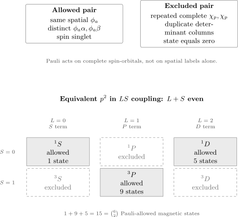
Top: two electrons may share a spatial orbital only through distinct spin-orbitals, while repeating one complete spin-orbital gives a zero determinant. Bottom: for two equivalent $p$ electrons, antisymmetry retains $^1S$, $^3P$, and $^1D$ and excludes the other naive $LS$ combinations. Their $1+9+5=15$ magnetic states exhaust $\binom{6}{2}$.

Equivalent Electrons

Electrons are equivalent in atomic spectroscopy when they belong to the same $n\ell$ subshell. They share the same radial and orbital angular labels before $m_\ell$ and spin are resolved. Equivalent electrons face stronger term restrictions than electrons in different subshells because exchanging them cannot be hidden in different radial labels.

Exchange parity of an equivalent pair

Couple two equal orbital angular momenta $\ell$ to total $L$. Clebsch–Gordan symmetry gives

$$P_{12}|(\ell\ell)LM_L\rangle =(-1)^{2\ell-L} |(\ell\ell)LM_L\rangle.$$

Because $2\ell$ is even,

$$\eta_{\mathrm{orb}}=(-1)^L.$$

For two spin-$1/2$ particles,

$$P_{12} \left| \left(\tfrac12\,\tfrac12\right) SM_S \right\rangle =(-1)^{S+1} \left| \left(\tfrac12\,\tfrac12\right) SM_S \right\rangle.$$

The singlet $S=0$ is antisymmetric and the triplet $S=1$ is symmetric. The product exchange parity is

$$\eta_{\mathrm{total}} =(-1)^{L+S+1}.$$

Fermionic antisymmetry requires $\eta_{\mathrm{total}}=-1$, so an equivalent $n\ell^2$ pair in pure $LS$ coupling must satisfy

$$L+S \quad\text{even}.$$

This compact rule is specific to two equivalent electrons with equal $\ell$. It should not be applied unchanged to arbitrary configurations.

The p-Squared Example

For $p^2$, each electron has $\ell=1$, so ordinary angular-momentum addition gives $L=0,1,2$ and $S=0,1$. Pauli antisymmetry removes half of the naive combinations:

$L$	Term letter	Singlet $S=0$	Triplet $S=1$
0	$S$	$^1S$ allowed	$^3S$ excluded
1	$P$	$^1P$ excluded	$^3P$ allowed
2	$D$	$^1D$ allowed	$^3D$ excluded

The allowed term-space dimensions are

$$\begin{aligned} ^1S:&\quad(2S+1)(2L+1)=1,\\ ^3P:&\quad(2S+1)(2L+1)=9,\\ ^1D:&\quad(2S+1)(2L+1)=5. \end{aligned}$$

Their sum is

$$1+9+5=15 =\binom{6}{2},$$

exactly the number of two-electron determinants in six $p$ spin-orbitals. This closure is a stringent check: no Pauli-allowed magnetic states are missing or counted twice.

Spin–orbit coupling later resolves $^3P$ into $J=0,1,2$ levels while preserving the total count $1+3+5=9$. Atomic Term Symbols owns that term-to-level hierarchy.

Why non-equivalent electrons differ

For a configuration such as $1s\,2s$, the radial orbitals differ. Symmetric and antisymmetric spatial combinations are both nonzero:

$$\begin{aligned} \psi_{\pm} ={}&\frac{1}{\sqrt2} \bigl[ \phi_{1s}(1)\phi_{2s}(2)\\ &\qquad\pm \phi_{2s}(1)\phi_{1s}(2) \bigr]. \end{aligned}$$

The symmetric spatial combination pairs with a singlet, and the antisymmetric combination pairs with a triplet. Thus helium’s $1s\,2s$ configuration supports both $^1S$ and $^3S$. Naive use of the equivalent-electron rule $L+S$ even would incorrectly delete the triplet.

Particles and Holes in One Subshell

A subshell of capacity $g$ has the same determinant count for $q$ electrons and $g-q$ electrons:

$$\binom{g}{q} =\binom{g}{g-q}.$$

Within an isolated nonrelativistic subshell, particle–hole conjugate configurations have the same allowed $LS$ term content. For a $p$ subshell:

Occupation	Determinants	Allowed terms
$p^0$, $p^6$	1	$^1S$
$p^1$, $p^5$	6	$^2P$
$p^2$, $p^4$	15	$^1S$, $^1D$, $^3P$
$p^3$	20	$^4S$, $^2D$, $^2P$

The dimensions close:

$$\begin{aligned} p^3:\quad 4+10+6 &=20\\ &=\binom{6}{3}. \end{aligned}$$

Particle–hole correspondence does not imply identical energies, radial relaxation, fine-structure order, or spectra for different atoms. It is a state-counting and angular-structure relation within the stated subshell model.

Shell Capacities

For a nonrelativistic subshell,

$$g_\ell=2(2\ell+1).$$

In ideal hydrogenic shell counting, $\ell=0,1,\ldots,n-1$, so

$$\begin{aligned} g_n &=\sum_{\ell=0}^{n-1}2(2\ell+1)\\ &=2n^2. \end{aligned}$$

The resulting capacities $2,8,18,32,\ldots$ describe the dimension of each ideal shell’s spin-orbital space. They do not say that real neutral atoms fill entire principal shells in that sequence. Multi-electron energies split by $\ell$, and neighboring principal shells overlap energetically.

Closed subshells

When every mode of an $n\ell$ subshell is occupied, there is only one determinant within that subshell. The complete set is invariant under spatial and spin rotations, giving

$$L=S=J=0$$

and even parity. Closed subshells therefore carry no open-shell angular momentum, although their electrons still contribute to charge density, screening, exchange, polarization, and correlation.

From Helium to Sodium

A short sequence separates what Pauli decides from what the Hamiltonian decides.

Helium

The $1s$ spatial orbital supplies two spin-orbitals. Helium can occupy both as $1s^2$, but only in the singlet coupling required by antisymmetry.

Lithium

The $1s$ spin-orbitals are already occupied in a simple $1s^2$ core. A third electron cannot enter either complete $1s$ mode. It must occupy another mode. The atomic Hamiltonian makes $2s$ the leading ground-state choice; Pauli alone does not prove that $2s$ lies below $2p$.

Neon and sodium

The $2p^6$ subshell closes the $n=2$ valence space in neon’s leading configuration. Sodium has one additional electron, whose leading ground configuration is $[\mathrm{Ne}]\,3s$. The recurrence of a one-electron-outside-a-closed-core pattern connects lithium and sodium chemically, but the actual orbital ordering and ionization energies depend on screening, penetration, and interactions.

What Creates Shell Structure?

The phrase “Pauli creates shells” is useful only when its ingredients are separated.

Ingredient	Structural role
nuclear Coulomb attraction	supplies bound atomic orbitals and a discrete spectrum
rotational symmetry	organizes one-electron states into angular-momentum multiplets
electron spin	doubles the nonrelativistic spatial-orbital capacity
fermionic antisymmetry	limits each complete spin-orbital to one electron and filters many-electron terms
electron–electron interaction	produces screening, direct and exchange energies, relaxation, and correlation
relativistic interactions	split $j$ subshells and alter heavy-atom ordering

Pauli exclusion is therefore necessary for the observed shell and periodic structure, but not sufficient to calculate it. A hypothetical system of charged bosons with the same one-body spectrum would not be forced to occupy distinct modes in this way, yet the fermionic capacity rule alone still cannot predict the energy ordering of real atoms.

Chemistry and Periodicity

Chemical periodicity reflects recurring open-subshell structures outside compact cores. Exclusion fixes the finite capacities that make those patterns recur:

• one electron outside a closed core gives alkali-like valence structure;
• one missing electron in a nearly closed $p$ subshell gives halogen-like hole structure;
• a closed valence subshell gives a particularly simple $J=0$ reference;
• partially filled $d$ and $f$ subshells support many Pauli-allowed terms and dense spectra.

Several additional ingredients are indispensable:

• screening and penetration determine effective radial binding;
• exchange and Coulomb integrals split allowed terms;
• Hund’s Rules estimate some ground-term orderings but are not Pauli exclusion;
• correlation and configuration mixing modify single-configuration pictures;
• molecular bonding and crystal fields replace isolated-atom symmetry by a different mode basis.

Thus “the periodic table follows from Pauli” is directionally right but incomplete. The periodic table follows from fermionic electrons governed by the electromagnetic Hamiltonian, with nuclear charge changing from element to element. Periodic Table from Quantum Mechanics assembles the capacities, screened energetics, ionization data, and chemical caveats into that larger explanation.

Spectroscopic Consequences

Pauli restrictions remove entire terms, not merely individual orbital-box arrangements. That has observable consequences:

• only Pauli-allowed levels appear in an atomic spectrum;
• closed subshells contribute $J=0$ and simplify the remaining valence coupling;
• equivalent-electron restrictions control level counts and partition functions;
• holes reproduce characteristic term patterns of complementary fillings;
• configuration mixing occurs only among basis states that already satisfy antisymmetry.

Absence of a line does not by itself prove Pauli exclusion, because transition selection rules, weak matrix elements, population, and detector sensitivity can also suppress lines. The atomic assignment combines state counting with energies, $J$, parity, magnetic response, and transition data.

Historical Perspective

Pauli formulated his exclusion rule in 1925 while trying to organize atomic shell closure and complex spectral multiplets. His original statement used a fourth two-valued electron degree of freedom before the modern interpretation of electron spin was fully established. The determinant formulation and the broader language of fermionic antisymmetry emerged with many-particle wave mechanics.

In modern relativistic theory, the spin–statistics theorem connects half-integer spin fields with fermionic statistics. That theorem is not proved within nonrelativistic atomic quantum mechanics. Atomic calculations take the electron’s fermionic exchange symmetry as an input and explore its consequences with extraordinary precision.

A Reliable Pauli Check

When testing an atomic state or configuration:

1. Specify complete one-electron modes. Include spin or relativistic spinor labels.
2. Check duplicate occupations. No complete fermionic mode may appear twice.
3. Antisymmetrize all electrons. Core and valence electrons are not distinguishable species.
4. Separate determinant and term labels. A valid determinant need not have definite $L$, $S$, or $J$.
5. Apply equivalent-electron restrictions. Naive angular-momentum addition can overcount terms.
6. Close the state count. Sum $(2L+1)(2S+1)$ or $(2J+1)$ and compare with the determinant dimension.
7. Declare the coupling scheme. $LS$ restrictions should not be transplanted blindly into a relativistic $jj$ basis.
8. Keep energy questions separate. Pauli determines admissibility, not the ordering of admissible states.

Common Mistakes

“No two electrons can be at the same point”

False. Exclusion forbids identical complete one-electron states. Opposite-spin components of a singlet can have nonzero probability density at equal spatial positions. For same-spin electrons, antisymmetry does force the spatial amplitude to vanish at coincidence.

“Two electrons in an orbital just point in opposite directions”

The arrows in an orbital box denote spin projections in a chosen basis. The paired state is an antisymmetric spin singlet, not two labeled classical rotors.

“Pauli is electron–electron Coulomb repulsion”

False. Neutral fermions obey exclusion, and charged bosons would still have Coulomb repulsion. Statistics and interaction are distinct inputs.

“Pauli gives the Aufbau order”

False. Pauli limits occupations once modes are chosen. It does not establish the Madelung sequence or decide whether $4s$ or $3d$ is lower for a particular atom or ion.

“All angular-momentum sums are allowed”

False for equivalent electrons. The $p^2$ combinations $^3S$, $^1P$, and $^3D$ fail antisymmetry even though ordinary vector addition permits their $L$ and $S$ values separately.

“Opposite spins are required in different orbitals”

False. Electrons in distinct spatial orbitals can form either singlet or triplet couplings when the corresponding spatial exchange symmetry is included.

“Fractional orbital occupation violates exclusion”

False. A superposition or mixed state can have fractional expectation values. The Pauli bound for a natural spin-orbital is $0\leq n_k\leq1$.

“Pauli exclusion and Pauli matrices are the same result”

They share Pauli’s name but answer different questions. Pauli matrices represent spin-$1/2$ operators; exclusion is the antisymmetry of identical fermions.

Exercises

Exercise 1: Atomic capacities

Derive the maximum occupations of $s$, $p$, $d$, and $f$ subshells. Then derive the ideal shell capacity $2n^2$. State one reason that this does not determine the ground configuration of every neutral atom.

Solution

For fixed $\ell$, there are $2\ell+1$ values of $m_\ell$ and two spin projections, so

$$g_\ell=2(2\ell+1).$$

For $\ell=0,1,2,3$, this gives $2,6,10,14$. In an ideal hydrogenic shell, $\ell$ runs from $0$ to $n-1$:

$$\begin{aligned} g_n &=2\sum_{\ell=0}^{n-1}(2\ell+1)\\ &=2n^2. \end{aligned}$$

Real multi-electron subshells are split by screening, penetration, exchange, correlation, and relativistic effects. Pauli fixes capacities but not their energetic order.

Exercise 2: Same spatial orbital

Show that two electrons in the same spatial orbital can form a singlet but not a triplet. Does this imply that their spatial coordinates can never coincide?

Solution

The product $\phi_a(\mathbf r_1)\phi_a(\mathbf r_2)$ is symmetric. Fermionic antisymmetry therefore requires the antisymmetric spin singlet:

$$\chi_{00} =\frac{1}{\sqrt2} \left( \alpha_1\beta_2-\beta_1\alpha_2 \right).$$

A triplet spin function is symmetric and would require the antisymmetric spatial combination

$$\phi_a(\mathbf r_1)\phi_a(\mathbf r_2) -\phi_a(\mathbf r_2)\phi_a(\mathbf r_1),$$

which vanishes identically. The allowed singlet spatial factor need not vanish at $\mathbf r_1=\mathbf r_2$, so equal spatial coordinates are not generally forbidden.

Exercise 3: Equivalent p-squared terms

Use the exchange parities $(-1)^L$ for the coupled orbital state and $(-1)^{S+1}$ for the coupled spin state to derive the Pauli condition for $p^2$. List the allowed terms and verify their state count.

Solution

The total exchange parity is

$$(-1)^L(-1)^{S+1} =(-1)^{L+S+1}.$$

Requiring it to equal $-1$ gives $L+S$ even. For $L=0,1,2$ and $S=0,1$, the allowed pairs are

$$(L,S)=(0,0),(1,1),(2,0),$$

corresponding to

$$^1S,\qquad ^3P,\qquad ^1D.$$

Their dimensions are $1$, $9$, and $5$, so

$$1+9+5=15=\binom{6}{2}.$$

Exercise 4: Particle–hole counting

Use binomial counting to show that $p^2$ and $p^4$ have equal determinant dimensions. Why does equal term content not imply identical spectra for, say, carbon and oxygen?

Solution

A $p$ subshell has six spin-orbitals, so

$$\binom{6}{2}=15, \qquad \binom{6}{4}=15.$$

Particle–hole conjugation within the isolated subshell gives the same $^1S$, $^1D$, and $^3P$ term types. Carbon and oxygen nevertheless have different nuclear charges, radial orbitals, screening, direct and exchange integrals, spin–orbit constants, correlation, and coupling to other configurations. State-space correspondence does not make their Hamiltonian matrices equal.

Exercise 5: Non-equivalent electrons

For one electron in $1s$ and one in $2s$, construct normalized symmetric and antisymmetric spatial combinations. Pair them with the correct spin states and identify the allowed $LS$ terms.

Solution

The spatial combinations are

$$\begin{aligned} \psi_{\pm} ={}&\frac{1}{\sqrt2} \bigl[ \phi_{1s}(1)\phi_{2s}(2)\\ &\qquad\pm \phi_{2s}(1)\phi_{1s}(2) \bigr]. \end{aligned}$$

$\psi_+$ is symmetric and must multiply the antisymmetric singlet. $\psi_-$ is antisymmetric and must multiply a symmetric triplet. Since both one-electron orbital angular momenta are zero, $L=0$ in either case. The allowed terms are therefore

$$^1S \quad\text{and}\quad ^3S.$$

Both exist because the distinct radial orbitals make the antisymmetric spatial combination nonzero.

Exercise 6: Number-operator bound

Using fermionic anticommutation, show that $\hat n_p=a_p^\dagger a_p$ satisfies $\hat n_p^2=\hat n_p$. What does this imply for an eigenvalue of $\hat n_p$ and for its expectation value in an arbitrary normalized state?

Solution

Use $a_pa_p^\dagger=1-a_p^\dagger a_p$:

$$\begin{aligned} \hat n_p^2 &=a_p^\dagger a_p a_p^\dagger a_p\\ &=a_p^\dagger \left(1-a_p^\dagger a_p\right) a_p\\ &=a_p^\dagger a_p -a_p^\dagger a_p^\dagger a_pa_p\\ &=\hat n_p, \end{aligned}$$

because $(a_p^\dagger)^2=a_p^2=0$. A projector has eigenvalues $0$ and $1$. For an arbitrary normalized state, its expectation lies in the convex interval

$$0\leq\langle\hat n_p\rangle\leq1.$$

The expectation may be fractional when the state is a superposition or mixture of different occupations.

Exercise 7: What decides lithium’s third electron?

In the independent central-field picture of lithium, explain separately why the third electron cannot join the two $1s$ electrons and why it occupies a $2s$ rather than a $2p$ orbital in the leading ground configuration.

Solution

The $1s$ spatial orbital supplies exactly two complete spin-orbitals, $1s\alpha$ and $1s\beta$. Once both are occupied, Pauli exclusion forbids a third $1s$ occupation.

Pauli does not compare $2s$ and $2p$ energies. Their ordering follows from the atomic Hamiltonian, especially penetration and screening in the self-consistent field, with interaction and correlation corrections. Thus exclusion forces the electron out of the closed $1s$ spin-orbital set, while energetics selects the leading $2s$ occupation.

Cross-Links

• Multi-Electron Atoms
• Electron Configurations
• Slater Determinants in Atoms
• jj Coupling
• Hund’s Rules
• Periodic Table from Quantum Mechanics
• Helium Atom
• Exchange and Correlation
• Atomic Term Symbols
• Central-Field Approximation
• Atomic Orbitals Revisited
• Pauli Exclusion Principle
• Spin and Spatial Wavefunctions
• Slater Determinants
• Occupation-Number Basis
• Fermionic Anticommutation Relations
• Reduced Density Matrices
• Historical Pauli Exclusion Principle
• Pauli Exclusion Revisited
• Spin–Statistics Preview

References

1. W. Pauli, “Über den Zusammenhang des Abschlusses der Elektronengruppen im Atom mit der Komplexstruktur der Spektren”, Zeitschrift für Physik 31, 765–783 (1925).
2. W. Pauli, “Exclusion Principle and Quantum Mechanics”, Nobel Lecture, 13 December 1946.
3. International Union of Pure and Applied Chemistry, “Pauli Exclusion Principle”, Compendium of Chemical Terminology, 5th ed., online version 5.0.0, 2025.
4. W. C. Martin and W. L. Wiese, “Atomic Spectroscopy: An Introduction”, in G. W. F. Drake, ed., Atomic, Molecular, and Optical Physics Handbook, AIP Press, 1996; NIST online revision.
5. J. C. Slater, “The Theory of Complex Spectra”, Physical Review 34, 1293–1322 (1929).
6. E. U. Condon and G. H. Shortley, The Theory of Atomic Spectra, Cambridge University Press, 1935.
7. R. D. Cowan, The Theory of Atomic Structure and Spectra, University of California Press, 1981.
8. W. R. Johnson, Atomic Structure Theory: Lectures on Atomic Physics, Springer, 2007.
9. C. J. Foot, Atomic Physics, Oxford University Press, 2005.
10. B. H. Bransden and C. J. Joachain, Physics of Atoms and Molecules, 2nd ed., Pearson, 2003.
11. E. H. Lieb and R. Seiringer, The Stability of Matter in Quantum Mechanics, Cambridge University Press, 2010.