Hund's Rules

Hund’s rules are an ordered set of approximate rules for predicting the lowest spectroscopic term and fine-structure level associated with a declared free-atom electron configuration in the $LS$-coupling regime. For one open subshell, their familiar form is:

1. Among allowed terms of the configuration, the term with the largest total spin $S$ usually lies lowest.
2. Among the terms with that largest $S$, the term with the largest total orbital angular momentum $L$ usually lies lowest.
3. Within the selected $LS$ term, the smallest allowed $J$ usually lies lowest when the open subshell is less than half filled, while the largest $J$ usually lies lowest when it is more than half filled.

The ordering is lexicographic. Rule 2 is applied only among terms surviving Rule 1, and Rule 3 is applied only after an $LS$ term has been selected. The rules do not replace antisymmetrization, determine the ground electron configuration, or provide exact energies.

Their best domain is a free atom or ion with one open subshell, a reasonably isolated configuration, and sufficiently good $LS$ coupling. Outside that domain they remain clues, not verdicts.

Canonical Scope

This page owns the atomic use, derivation, and limitations of Hund’s three term-ordering rules:

• what each rule predicts and the order in which it is applied;
• the distinction from Pauli exclusion, orbital filling, and the Aufbau or Madelung heuristic;
• the fixed-orbital exchange model behind the maximum-spin tendency;
• why relaxed atomic energies require more care than the phrase “exchange lowers the energy” suggests;
• the stretched-state construction of maximum $S$ and maximum $L$;
• particle–hole symmetry across half filling;
• the spin–orbit derivation of the third rule;
• worked $p^q$ and $d^q$ ground-term assignments;
• configuration, coupling, field, and correlation failure modes.

Neighboring pages retain their canonical subjects. Pauli Principle in Atoms determines which terms are allowed by antisymmetry. Electron Configurations owns subshell occupations and the limitations of filling rules. Atomic Term Symbols owns notation. Exchange and Correlation owns direct, exchange, and correlation accounting. LS Coupling owns the coupling regime and Landé diagnostics, while jj Coupling owns the complementary relativistic-subshell limit.

What the Rules Do and Do Not Order

Consider a central-field configuration

$$\mathcal C = \prod_a(n_a\ell_a)^{q_a}.$$

Several different objects can be associated with this one label:

• determinants with specified one-electron magnetic occupations;
• antisymmetric configuration-state functions with specified $L$ and $S$;
• terms labeled by $\gamma\,{}^{2S+1}L^\pi$;
• fine-structure levels labeled by $J$;
• exact eigenstates that may mix several configurations and terms.

Hund’s first two rules compare terms within a declared configuration. The third compares $J$ levels within the selected term. A useful ideal hierarchy is

$$\begin{aligned} \Delta E_{\mathrm{config}} &\gg \Delta E_{\mathrm{term}},\\ \Delta E_{\mathrm{term}} &\gg \Delta E_{\mathrm{fs}}. \end{aligned}$$

The first two rules summarize regularities in the electrostatic term splittings. The third uses the weaker spin–orbit ordering. If these scales overlap, the labels themselves can mix and the three-step procedure loses accuracy.

Four ideas that are often conflated

1. Pauli exclusion is a kinematic consequence of fermionic antisymmetry. It forbids repeated complete spin-orbitals and removes inadmissible terms.
2. A configuration or filling rule proposes which subshell occupations should be compared for the ground state.
3. Hund’s rules rank allowed terms and levels, approximately, after a configuration has been declared.
4. Hamiltonian diagonalization supplies the actual energies and eigenvectors for the model being used.

The classroom instruction “put one electron in each degenerate orbital before pairing” is a determinant-level way to construct a maximum-$M_S$ representative of Rule 1. It is not the complete content of all three rules. It also assumes a degenerate or nearly degenerate orbital set; a sufficiently large orbital-energy splitting can favor pairing.

Free atoms, not arbitrary environments

The quantum numbers $L$, $S$, and $J$ refer to rotational symmetry of an isolated atom. A crystal field can split orbital components and quench $L$; a molecule has different spatial symmetry and often different equilibrium geometries for different spin states. Molecular Hund cases are angular-momentum coupling schemes, not these atomic term-ordering rules.

Rule 1: Maximum Spin

Within a fixed configuration, the allowed term with the largest $S$ commonly has the lowest electrostatic energy. Its multiplicity is

$$2S+1.$$

“Parallel spins” is shorthand for the stretched component with $M_S=S$. A rotationally invariant term also contains the other $M_S=-S,\ldots,S$ components. The rule does not assign classical arrows permanently pointing in one laboratory direction.

Two-electron fixed-orbital model

Let $a$ and $b$ be orthonormal spatial orbitals. The normalized symmetric and antisymmetric spatial functions are

$$\Psi_\pm(1,2) = \frac{1}{\sqrt2} \left[ a(1)b(2) \pm b(1)a(2) \right].$$

The spin singlet requires the symmetric spatial function $\Psi_+$, while the spin triplet requires the antisymmetric spatial function $\Psi_-$. For the Coulomb interaction

$$V_{12} = \frac{e^2}{4\pi\epsilon_0r_{12}},$$

define the direct and exchange integrals

$$\begin{aligned} J_{ab} &= \iint |a(1)|^2 V_{12} |b(2)|^2 \,d1\,d2,\\ K_{ab} &= \iint a^*(1)b^*(2) V_{12} b(1)a(2) \,d1\,d2. \end{aligned}$$

With the same one-electron orbitals in both states,

$$\begin{aligned} \langle\Psi_+|V_{12}|\Psi_+\rangle &=J_{ab}+K_{ab},\\ \langle\Psi_-|V_{12}|\Psi_-\rangle &=J_{ab}-K_{ab}. \end{aligned}$$

Thus the fixed-orbital singlet–triplet separation is

$$E_{\mathrm S}-E_{\mathrm T} = 2K_{ab}.$$

For the positive Coulomb kernel, $K_{ab}$ is nonnegative. In this restricted model the triplet is therefore lower. The antisymmetric spatial function also vanishes at equal coordinates,

$$\Psi_-(\mathbf r,\mathbf r)=0,$$

which is the two-electron signature of the same-spin exchange hole.

The important energy-accounting caveat

The fixed-orbital derivation is exact for the trial functions just declared. It does not prove that a fully optimized high-spin atom has a smaller expectation value of electron–electron repulsion than the corresponding low-spin atom.

When each term is allowed to relax, its orbitals, kinetic energy, electron–nucleus attraction, direct energy, exchange energy, and correlation energy all change. Virial-theorem and multiconfiguration analyses of second- and third-row $p$ atoms find that the high-spin stabilization can be realized through stronger electron–nucleus attraction after radial contraction, even when the electron–electron repulsion and kinetic energy increase.

The trustworthy summary is:

Antisymmetry creates spin-dependent spatial structure. In a common fixed-orbital model this appears as a lowering by exchange integrals; in a relaxed atom, the final term separation is a total-energy balance.

This is why “electrons with parallel spins repel less” is too literal. The Coulomb operator is spin independent, and no additional exchange force has been added.

Why Pauli is not Rule 1

Pauli antisymmetry determines the admissible Hilbert space. It can force two electrons in the same spatial orbital into a singlet, as in $1s^2$. For electrons in distinct orbitals, both singlet and triplet terms may be allowed. Hund’s first rule then predicts an energy ordering between allowed terms; it is not an exclusion law.

Rule 2: Maximum Orbital Angular Momentum

After selecting the maximum-$S$ terms, the one with the largest $L$ commonly lies lowest. The ordering applies to total orbital angular momentum,

$$\mathbf L=\sum_i\mathbf l_i,$$

not to a sum of one-electron orbital energies.

For one equivalent open subshell, electrostatic term energies can be organized schematically as

$$E(\alpha LS) = E_{\mathrm{av}} + \sum_{k>0} f_k(\alpha LS)F^k.$$

Here $E_{\mathrm{av}}$ is a configuration average, the $F^k$ are radial Slater–Condon integrals, and the dimensionless $f_k$ are angular coefficients fixed by the antisymmetric term. Rule 2 summarizes a frequent pattern of these angular coefficients. It is not a universal centrifugal-energy theorem proportional to $L(L+1)$.

Why the common orbital picture is limited

A stretched maximum-$L$ component places the parallel-spin electrons in the largest available $m_\ell$ values. This construction is excellent for finding the candidate term. Its angular density and exchange correlations often support efficient electron avoidance, but statements such as “the electrons orbit in the same direction and stay farther apart” are classical pictures, not derivations.

The actual comparison uses matrix elements of the Coulomb Hamiltonian. Different radial functions, several open subshells, configuration interaction, and unusually large $L$ can invalidate the simple ordering.

Equivalent-Subshell Construction

Let $q$ electrons occupy one $n\ell$ subshell. The number of spatial orbitals is

$$m=2\ell+1,$$

and the spin-orbital capacity is

$$g=2m=4\ell+2.$$

Half filling occurs at $q=m$, not at $q=g/2$ as a separate condition; these are the same number.

Maximum spin

For $q\leq m$, place the electrons in distinct $m_\ell$ orbitals with the same spin projection. Then

$$S_{\max}=\frac q2.$$

For $q>m$, use the equivalent hole description with

$$q_{\mathrm h}=g-q.$$

The compact result is

$$q_*=\min(q,g-q), \qquad S_{\max}=\frac{q_*}{2}.$$

The electron and hole configurations $n\ell^q$ and $n\ell^{g-q}$ support the same set of $L$ and $S$ terms, although their fine-structure ordering reverses across half filling.

Maximum orbital angular momentum

For the stretched maximum-spin component with $q_*\leq m$, occupy

$$m_\ell = \ell,\ell-1,\ldots,\ell-q_*+1.$$

The largest projection is

$$\begin{aligned} M_{L,\max} &= \sum_{r=0}^{q_*-1}(\ell-r)\\ &= q_*\ell - \frac{q_*(q_*-1)}{2}. \end{aligned}$$

A state with the largest possible projection must belong to a term with

$$L_{\max}=M_{L,\max}.$$

Combining Rules 1 and 2 therefore predicts, for one equivalent open subshell,

$$\begin{aligned} S_{\mathrm H} &= \frac{q_*}{2},\\ L_{\mathrm H} &= q_*\ell - \frac{q_*(q_*-1)}{2}. \end{aligned}$$

The subscript $\mathrm H$ marks the Hund-rule candidate, not an exact theorem about the full atomic ground state.

Quick checks

• $p^2$: $q_*=2$, so $S_{\mathrm H}=1$ and $L_{\mathrm H}=1$, giving $\,{}^3P$.
• $p^3$: $q_*=3$, so $S_{\mathrm H}=3/2$ and $L_{\mathrm H}=0$, giving $\,{}^4S$.
• $d^2$: $q_*=2$, so $S_{\mathrm H}=1$ and $L_{\mathrm H}=3$, giving $\,{}^3F$.
• $d^5$: $q_*=5$, so $S_{\mathrm H}=5/2$ and $L_{\mathrm H}=0$, giving $\,{}^6S$.
• $f^2$: $q_*=2$, so $S_{\mathrm H}=1$ and $L_{\mathrm H}=5$, giving $\,{}^3H$.

These formulas identify the term selected by the first two rules. They do not enumerate all allowed terms, which still requires antisymmetry and state counting.

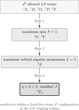
For a fixed $d^2$ configuration in $LS$ coupling, Rule 1 retains the triplets, Rule 2 selects $\,{}^3F$, and Rule 3 selects $J=2$ because the $d$ subshell is less than half filled. The diagram is a prediction workflow, not a proof of the level energies.

Rule 3: Ordering the J Levels

Once Rules 1 and 2 have selected an $LS$ term, total angular momentum can take the values

$$J=|L-S|,\ldots,L+S.$$

In an isolated term with weak fine structure, the leading effective interaction is often written

$$H_{\mathrm{so}}^{\mathrm{eff}} = A\,\mathbf L\cdot\mathbf S.$$

Its first-order level energy is

$$\begin{aligned} E_J-E_{LS} &= \frac A2 \bigl[J(J+1)\\ &\qquad -L(L+1)-S(S+1)\bigr]. \end{aligned}$$

Adjacent levels obey

$$E_J-E_{J-1}=AJ.$$

Therefore:

• if $A>0$, energy increases with $J$ and the smallest $J=|L-S|$ lies lowest;
• if $A<0$, energy decreases with $J$ and the largest $J=L+S$ lies lowest.

For a single equivalent open subshell in ordinary $LS$ coupling, the effective sign commonly follows the filling:

$$J_{\mathrm H} = \begin{cases} |L_{\mathrm H}-S_{\mathrm H}|, &q<2\ell+1,\\[4pt] S_{\mathrm H}, &q=2\ell+1,\\[4pt] L_{\mathrm H}+S_{\mathrm H}, &q>2\ell+1. \end{cases}$$

At exact half filling, the maximum-spin term of one equivalent subshell has $L_{\mathrm H}=0$, so only $J=S_{\mathrm H}$ occurs. There is no multiplet ordering left for Rule 3 to decide.

Particle–hole reversal

Configurations $n\ell^q$ and $n\ell^{g-q}$ have the same allowed $L$ and $S$ terms. Their electron and hole descriptions, however, reverse the spin–orbit ordering within corresponding terms. Thus

$$d^2 \longleftrightarrow d^8$$

share the Hund candidate $\,{}^3F$, but Rule 3 predicts

$$\begin{aligned} d^2&:\quad{}^3F_2,\\ d^8&:\quad{}^3F_4. \end{aligned}$$

This is the logic behind the less-than-half-filled and more-than-half-filled wording. It is not a statement that the magnitude of every fine-structure interval is the same for electron and hole partners.

Worked d² interval pattern

For $\,{}^3F$, one has $L=3$ and $S=1$, so $J=2,3,4$. The effective shifts are

$$\begin{aligned} \Delta E_2&=-4A,\\ \Delta E_3&=-A,\\ \Delta E_4&=3A. \end{aligned}$$

For $d^2$, Rule 3 corresponds to $A>0$, so $J=2$ lies lowest. The interval ratio is

$$\frac{E_4-E_3}{E_3-E_2} = \frac43.$$

This is the isolated-term Landé interval prediction. Real intervals need not obey it exactly because spin–spin, spin–other-orbit, configuration interaction, and intermediate coupling also contribute. LS Coupling owns the full diagnostic.

Worked Ground-Term Examples

The following examples use closed cores with $L=S=J=0$, so only the open subshell needs to be considered. NIST evaluated ground-level designations provide the empirical check.

Carbon: p²

Neutral carbon has the leading ground configuration

$$1s^2\,2s^2\,2p^2.$$

For $p^2$, $\ell=1$, $q=2$, $g=6$, and $q_*=2$. The first two rules give

$$S_{\mathrm H}=1, \qquad L_{\mathrm H}=1,$$

so the candidate term is $\,{}^3P$. The subshell is less than half filled because $2<3$, hence

$$J_{\mathrm H}=|1-1|=0.$$

The parity is even:

$$\pi=(-1)^{2\ell}=+1.$$

The prediction is

$$1s^2\,2s^2\,2p^2\;{}^3P_0,$$

which is the evaluated C I ground level.

Nitrogen: p³

Neutral nitrogen has a half-filled $2p^3$ subshell. The three parallel-spin electrons occupy

$$m_\ell=1,0,-1$$

in the stretched determinant, giving

$$S_{\mathrm H}=\frac32, \qquad L_{\mathrm H}=0.$$

Thus

$$J_{\mathrm H}=\frac32.$$

Three $p$ electrons have odd parity, so the predicted ground level is

$$1s^2\,2s^2\,2p^3\;{}^4S^\circ_{3/2}.$$

This is the evaluated N I ground level. The result also shows why the letter $S$ in a term symbol does not mean that the electrons occupy $s$ orbitals: it denotes total $L=0$.

Oxygen: p⁴

The open $2p^4$ subshell of neutral oxygen is particle–hole conjugate to $p^2$. Therefore Rules 1 and 2 again give

$$S_{\mathrm H}=1, \qquad L_{\mathrm H}=1,$$

and the term is $\,{}^3P$. Now $4>3$, so the subshell is more than half filled and Rule 3 selects

$$J_{\mathrm H}=L+S=2.$$

The evaluated O I ground level is

$$1s^2\,2s^2\,2p^4\;{}^3P_2.$$

Carbon and oxygen therefore have the same ground term but opposite ends of the $J=0,1,2$ multiplet as their ground levels.

Titanium and nickel: d² and d⁸

The leading neutral-titanium ground configuration contains $3d^2\,4s^2$. The closed $4s^2$ pair contributes zero angular momentum, and the $d^2$ open subshell gives

$${}^3F_2.$$

The NIST level compilation places the other members of this term at higher energy in the order

$$J=2,\ 3,\ 4.$$

Neutral nickel’s leading ground configuration contains $3d^8\,4s^2$. The $d^8$ open subshell is the two-hole partner of $d^2$, so it has the same $\,{}^3F$ term but the opposite third-rule ordering:

$${}^3F_4.$$

The evaluated Ti I and Ni I ground designations thus give a direct electron–hole comparison.

A Reliable Assignment Workflow

Use the following sequence when applying the rules.

1. Specify the species and Hamiltonian. Distinguish the neutral atom from its ions and state whether a free-atom, field-free model is intended.
2. Declare the configuration. Do not use Hund’s rules to choose between competing configurations.
3. Identify the open subshells. Closed subshells contribute $L=S=J=0$.
4. Construct the allowed terms. Enforce Pauli antisymmetry before ordering anything.
5. Apply Rule 1. Retain the largest allowed $S$.
6. Apply Rule 2. Among those terms, retain the largest allowed $L$.
7. List the allowed $J$ values. Use $J=|L-S|,\ldots,L+S$.
8. Apply Rule 3 only in its domain. For one equivalent subshell in $LS$ coupling, use its position relative to half filling.
9. Compute parity independently. For a configuration,

$$\pi=(-1)^{\sum_i\ell_i}.$$

10. Verify the assignment. Compare with evaluated spectroscopy and inspect calculated eigenvector compositions when mixing is possible.

This workflow keeps a useful mnemonic from silently doing work that belongs to antisymmetry or dynamics.

Limitations and Exceptions

Hund’s rules are remarkably successful for many free-atom ground configurations, but no variational theorem says that they must hold for every Hamiltonian or every configuration.

Configuration mixing

The rules rank terms associated with a declared configuration. If two configurations of the same exact $J^\pi$ are close, the Hamiltonian can mix them:

$$|\Psi_{\nu J\pi}\rangle = \sum_a c_a^{(\nu)} |\mathcal C_a\alpha_aLSJ\pi\rangle.$$

The resulting eigenstate may not possess a single well-defined configuration, $L$, or $S$. A dominant-component label can remain useful, but its weight should be reported.

Several open subshells

The compact formulas using $q_*=\min(q,g-q)$ apply to one equivalent open subshell. With two or more open subshells, one must first determine parent terms and their coupling. Kutzelnigg and Morgan’s review emphasizes that exceptions to simple first- and second-rule forms occur especially in configurations with multiple open subshells carrying nonzero orbital angular momentum and in some large-$L$ cases.

Relativistic and intermediate coupling

The first two rules assume that $L$ and $S$ organize the electrostatic terms before fine structure is applied. In a heavy atom, strong one-electron spin–orbit splitting can favor a jj-coupled description. Then individual $j$ occupations and subshell parents can be more informative than one pure $LS$ term.

Even when $LS$ labels remain recognizable, same-$J^\pi$ mixing can move levels away from the third-rule pattern. A statement such as “more than half filled, therefore largest $J$” is not reliable unless the isolated-term and coupling assumptions have been checked.

Excited configurations and accidental near-degeneracy

The rules are most dependable as ground-term guides. They do not globally sort terms from different configurations, and rare reversals occur among excited states. Small denominators amplify interactions that a broad energy-scale argument would otherwise treat as perturbations.

Explicit calculations along isoelectronic sequences provide documented examples of excited-state failures and changing assignments. Such cases are evidence against overextending the rules, not failures of antisymmetry or angular-momentum algebra.

Orbital relaxation and correlation

The fixed-orbital exchange formula explains an important tendency, but optimized terms use different radial functions and correlation patterns. The energy components

$$T,\qquad V_{\mathrm{en}},\qquad V_{\mathrm{ee}}$$

can each move in a direction that contradicts a one-sentence “less repulsion” story while their sum still obeys Rule 1. Only total energies computed with a consistent Hamiltonian decide the ordering.

External fields, solids, and molecules

Electric, magnetic, crystal, and ligand fields can compete with the atomic electrostatic and spin–orbit scales. In a ligand field, the cost of occupying a higher crystal-field orbital can exceed the intra-atomic high-spin preference and produce a low-spin state. This is not a violation of an exact atomic law; it is a different Hamiltonian outside the free-atom assumptions.

Hund coupling in many-body models

Multi-orbital Hubbard and Kanamori models often contain a parameter called Hund coupling or Hund exchange, usually written $J_{\mathrm H}$. It lowers selected high-spin local multiplets and may include spin-flip and pair-hopping terms required by rotational invariance.

That model parameter is related to the same atomic interaction physics, but it is not identical to the three spectroscopic rules. In particular, a local $J_{\mathrm H}$ does not by itself reproduce free-atom Rule 2 or the less-than-half-filled versus more-than-half-filled fine-structure ordering. See the Hubbard Model for the lattice-model boundary.

Common Mistakes

• Using Hund’s rules to determine the electron configuration. They order terms after a configuration has been declared.
• Treating maximum spin as Pauli exclusion. Pauli removes forbidden states; Rule 1 compares energies of allowed states.
• Applying Rule 2 before Rule 1. Largest $L$ is chosen only among the maximum-$S$ terms.
• Applying Rule 3 across different terms. It orders $J$ levels within one selected $LS$ term.
• Calling the rules exact. They are empirical and asymptotically motivated regularities with identifiable failure modes.
• Saying parallel spins feel a weaker Coulomb force. The Coulomb operator is spin independent; antisymmetry changes the spatial state.
• Assuming the optimized high-spin state always has lower electron–electron repulsion. Relaxation changes all energy components.
• Counting half filling incorrectly. An $n\ell$ subshell is half filled at $q=2\ell+1$.
• Using electron rather than hole counting above half filling. The $L,S$ term structure is often easiest to obtain from $q_{\mathrm h}=4\ell+2-q$ holes.
• Applying free-atom rules unchanged in a ligand field or molecule. The relevant symmetry and energy hierarchy have changed.
• Confusing Hund’s rules with molecular Hund cases or a many-body $J_{\mathrm H}$ parameter. These are related names for distinct constructions.

Exercises

Exercise 1: Separate the four layers

Classify each statement as Pauli exclusion, a configuration-filling heuristic, a Hund-rule prediction, or a Hamiltonian result:

1. no complete spin-orbital can be occupied twice;
2. neutral carbon is represented first by $1s^2\,2s^2\,2p^2$;
3. within $2p^2$, the $\,{}^3P$ term is predicted below the singlet terms;
4. the measured C I ground level has energy defined as zero in an evaluated table.

Solution

Statement 1 is Pauli exclusion in an occupation basis. Statement 2 is a configuration assignment supported by central-field energetics and spectroscopy; a filling heuristic may propose it, but Hund’s rules do not derive it.

Statement 3 is the combined Rule 1 and Rule 2 prediction within the declared configuration. Statement 4 is an empirical Hamiltonian-spectrum result represented in an evaluated database.

The distinctions matter because only the first statement is an exact kinematic restriction. The others involve increasingly detailed dynamical information.

Exercise 2: Derive the p² ground level

Use the equivalent-subshell formulas and all three rules to predict the lowest level of $p^2$. Include parity.

Solution

For $\ell=1$, the capacity is

$$g=4\ell+2=6.$$

With $q=2$,

$$q_*=\min(2,4)=2.$$

Therefore

$$S_{\mathrm H}=\frac{q_*}{2}=1,$$

and

$$\begin{aligned} L_{\mathrm H} &= q_*\ell - \frac{q_*(q_*-1)}{2}\\ &= 2-\frac{2}{2}=1. \end{aligned}$$

The term is $\,{}^3P$. Since $q=2<3$, Rule 3 selects

$$J=|L-S|=0.$$

Two $p$ electrons have parity

$$(-1)^{2\ell}=+1.$$

The predicted lowest level is therefore

$${}^3P_0$$

with even parity.

Exercise 3: Half filling and particle–hole symmetry

Predict the Hund-rule levels for $p^3$ and $p^4$. Explain why the first has only one $J$ value while the second reverses the $p^2$ third-rule ordering.

Solution

For $p^3$, $q_*=3$. Thus

$$S_{\mathrm H}=\frac32,$$

and

$$L_{\mathrm H} = 3(1)-\frac{3\cdot2}{2} =0.$$

The term is $\,{}^4S$. Because $L=0$, only

$$J=S=\frac32$$

occurs. Its parity is odd, so the level is $\,{}^4S^\circ_{3/2}$.

For $p^4$, use two holes. The term is again $\,{}^3P$, but the electron subshell is more than half filled. Rule 3 therefore selects

$$J=L+S=2.$$

The level is $\,{}^3P_2$ with even parity. The allowed $L,S$ terms match $p^2$, while particle–hole conjugation reverses which end of the $J$ multiplet lies lowest.

Exercise 4: The d² cascade

The allowed $d^2$ terms include

$${}^1S,\quad {}^1D,\quad {}^1G,\quad {}^3P,\quad {}^3F.$$

Apply the rules in order and predict the lowest level.

Solution

Rule 1 retains the triplets,

$${}^3P \qquad\text{and}\qquad {}^3F,$$

because they have $S=1$. Rule 2 chooses the larger orbital angular momentum, $L=3$, so the term is $\,{}^3F$.

For a $d$ subshell, half filling is $q=2\ell+1=5$. Since $q=2<5$, Rule 3 chooses the smallest allowed total,

$$J=|L-S|=|3-1|=2.$$

The predicted lowest level is

$${}^3F_2.$$

Exercise 5: The d⁸ hole partner

Use particle–hole symmetry to predict the lowest $d^8$ level. Compare it with $d^2$.

Solution

A $d$ subshell has capacity

$$g=4\ell+2=10.$$

The $d^8$ configuration has

$$q_{\mathrm h}=10-8=2$$

holes, so Rules 1 and 2 give the same $\,{}^3F$ term as $d^2$. Because the electron subshell is more than half filled, Rule 3 selects the largest total,

$$J=L+S=3+1=4.$$

Thus

$$d^2\longrightarrow{}^3F_2, \qquad d^8\longrightarrow{}^3F_4.$$

The terms agree, while the fine-structure ordering reverses.

Exercise 6: Exchange energy and its limit

Two orthonormal fixed orbitals have exchange integral $K_{ab}=0.40\ \mathrm{eV}$. What singlet–triplet splitting does the fixed-orbital model predict? Does this imply that the fully optimized triplet must have a lower electron–electron repulsion expectation than the fully optimized singlet?

Solution

The fixed-orbital result is

$$E_{\mathrm S}-E_{\mathrm T} = 2K_{ab} = 0.80\ \mathrm{eV}.$$

Thus the triplet is lower by $0.80\ \mathrm{eV}$ in that restricted comparison.

The second conclusion does not follow. Once each term is optimized, its orbitals and correlation change. The triplet can have a larger electron–electron repulsion and kinetic energy but a sufficiently stronger electron–nucleus attraction to produce the lower total energy. Only a comparison of total energies under the same Hamiltonian determines the ordering.

Exercise 7: Diagnose when the rules are insufficient

A heavy atom has two open subshells. A calculation finds three same-$J^\pi$ basis components with weights $44\%$, $33\%$, and $15\%$, split between LS and jj parentage. The observed magnetic factor differs by $25\%$ from the pure-LS prediction. Is a Hund-rule ground-level assignment by itself trustworthy?

Solution

No. The system violates several assumptions behind a standalone Hund assignment:

• more than one open subshell makes the simple equivalent-subshell formulas inapplicable;
• no component dominates strongly;
• mixed LS and jj parentage signals intermediate coupling;
• the magnetic factor directly contradicts a pure-LS description.

Hund’s rules may still suggest useful basis components, but the assignment should come from diagonalizing the declared Hamiltonian in the full fixed-$J^\pi$ space and comparing energies, eigenvector compositions, magnetic factors, and transitions. Reporting only one pure term label would hide the relevant physics.

Key Takeaways

• Hund’s rules approximately rank terms and levels within a declared free-atom configuration; they do not choose the configuration.
• Rule 1 maximizes $S$, Rule 2 then maximizes $L$, and Rule 3 orders $J$ within that selected term.
• Pauli antisymmetry determines which terms exist before any energy rule is applied.
• The fixed-orbital exchange calculation gives $E_{\mathrm S}-E_{\mathrm T}=2K_{ab}$, but optimized atomic term energies involve relaxation and correlation across all energy components.
• For one $n\ell^q$ subshell, $q_*=\min(q,4\ell+2-q)$ gives $S_{\mathrm H}=q_*/2$ and the stretched-state value of $L_{\mathrm H}$.
• Electron–hole partners share the same $L,S$ terms but reverse the usual third-rule ordering across half filling.
• The third rule follows from the sign of an effective $A\mathbf L\cdot\mathbf S$ interaction, not from an independent exclusion principle.
• Multiple open subshells, configuration mixing, strong spin–orbit coupling, external fields, and orbital relaxation can defeat simple applications.
• Molecular Hund cases and many-body Hund coupling are related terminology, not synonyms for the three atomic rules.

Cross-Links

• Magnetic Moments in Matter uses the free-ion $L,S,J$ term as a baseline, then tests how crystal fields, covalency, itinerancy, and the probe window change the material moment.
• Multi-Electron Atoms
• Electron Configurations
• Periodic Table from Quantum Mechanics
• Pauli Principle in Atoms
• Exchange and Correlation
• Slater Determinants in Atoms
• LS Coupling
• jj Coupling
• Atomic Term Symbols
• Central-Field Approximation
• Atomic Orbitals Revisited
• Fine Structure
• Atomic Selection Rules
• Ferrimagnetism — uses atomic spin and orbital moments as the ionic baseline for unequal magnetic sublattices.
• Angular Momentum Coupling Schemes
• Hubbard Model
• AMO Physics Roadmap

References

1. F. Hund, “Zur Deutung verwickelter Spektren, insbesondere der Elemente Scandium bis Nickel”, Zeitschrift für Physik 33, 345–371 (1925).
2. W. C. Martin and W. L. Wiese, “Atomic Spectroscopy: An Introduction”, in G. W. F. Drake, ed., Atomic, Molecular, and Optical Physics Handbook, AIP Press, 1996; NIST online revision updated 2025.
3. A. Kramida, Yu. Ralchenko, J. Reader, and the NIST ASD Team, NIST Atomic Spectra Database, version 5.12, National Institute of Standards and Technology, data content updated November 2024, DOI: 10.18434/T4W30F, accessed 2026-07-21.
4. NIST Physical Measurement Laboratory, evaluated ground-state pages for C I, N I, O I, Ti I, and Ni I, accessed 2026-07-21.
5. E. U. Condon and G. H. Shortley, The Theory of Atomic Spectra, Cambridge University Press, 1935.
6. J. C. Slater, Quantum Theory of Atomic Structure, Vols. I–II, McGraw–Hill, 1960.
7. R. D. Cowan, The Theory of Atomic Structure and Spectra, University of California Press, 1981.
8. W. Kutzelnigg and J. D. Morgan III, “Hund’s Rules”, Zeitschrift für Physik D 36, 197–214 (1996).
9. J. D. Morgan III and W. Kutzelnigg, “Hund’s Rules, the Alternating Rule, and Symmetry Holes”, Journal of Physical Chemistry 97, 2425–2434 (1993).
10. T. Oyamada, K. Hongo, Y. Kawazoe, and H. Yasuhara, “Unified Interpretation of Hund’s First and Second Rules for 2p and 3p Atoms”, Journal of Chemical Physics 133, 164113 (2010).
11. G. Friesecke and B. D. Goddard, “Atomic Structure via Highly Charged Ions and Their Exact Quantum States”, Physical Review A 81, 032516 (2010).
12. W. R. Johnson, Atomic Structure Theory: Lectures on Atomic Physics, Springer, 2007.
13. I. I. Sobelman, Atomic Spectra and Radiative Transitions, 2nd ed., Springer, 1992.