Slater Determinants in Atoms

An atomic Slater determinant specifies which complete one-electron spin-orbitals are occupied in a chosen atomic orbital basis. It is an antisymmetric many-electron basis state and should not be identified by default with an electron configuration, spectroscopic term, or exact atomic level.

In a nonrelativistic central-field basis, a spin-orbital may be labeled

$$\chi_{n\ell m_\ell m_s}(x) = \frac{P_{n\ell}(r)}{r} Y_{\ell m_\ell}(\Omega) \eta_{m_s}(\sigma).$$

Choosing $N$ distinct spin-orbitals produces a determinant

$$|D_I\rangle = a_{i_1}^\dagger a_{i_2}^\dagger\cdots a_{i_N}^\dagger|0\rangle,$$

where one fixed ordering convention for the creation operators is understood. In a complex spherical-harmonic basis, this state has definite particle number, parity, $M_L$, and $M_S$. It need not have definite total $L$ or $S$.

Atomic structure calculations therefore use two complementary bases:

• determinants, which make occupation and antisymmetry explicit;
• configuration-state functions, which combine determinants to carry declared angular-momentum and parity labels.

The transformation between them is a change of basis inside the same antisymmetric state space. It does not add a new interaction or physical approximation by itself.

Canonical Scope

This page owns the practical atomic translation among:

• complete atomic spin-orbitals and their occupations;
• determinant notation and phase conventions;
• determinant quantum numbers $M_L$, $M_S$, and parity;
• configurations, determinants, microstates, and their counting;
• configuration-state functions, or CSFs;
• symmetry adaptation with $L^2$, $S^2$, $J^2$, and ladder operators;
• the relation between determinant bases and atomic term symbols;
• determinant connectivity under one- and two-electron operators;
• nonrelativistic and relativistic atomic basis choices.

Slater Determinants is the canonical home for determinant construction, normalization, nonorthogonal orbitals, and elementary coordinate-space examples. Electron Configurations owns occupation notation, Aufbau caveats, configuration mixing, and the interpretation of leading configuration weights. Pauli Principle in Atoms owns equivalent-electron restrictions and the allowed-term counting for configurations such as $p^2$. Atomic Term Symbols owns the grammar and interpretation of spectroscopic labels. LS Coupling owns the physical regime in which the resulting $L$ and $S$ labels organize atomic levels.

Atomic Spin-Orbitals

The complete one-electron label

The determinant must be built from complete one-particle states. In the nonrelativistic position-spin representation,

$$x=(\mathbf r,\sigma),$$

and a central-field spin-orbital carries

$$i=(n,\ell,m_\ell,m_s).$$

Two electrons may occupy the same spatial orbital $n\ell m_\ell$ provided they occupy different complete spin-orbitals, usually distinguished by $m_s=\pm1/2$. Repeating the same complete spin-orbital makes the determinant vanish.

For orthonormal radial functions, spherical harmonics, and spin functions,

$$\langle\chi_i|\chi_j\rangle = \delta_{ij}.$$

Distinct occupation patterns then produce orthonormal determinants.

Complex and real orbital bases

The statement that a determinant has definite $M_L$ assumes that each spatial orbital is an eigenfunction of $L_z$, as the complex spherical harmonics $Y_{\ell m}$ are. Real $p_x,p_y,p_z$ or real $d$ orbitals are linear combinations of different $m_\ell$ values. A determinant built from them can remain a perfectly valid antisymmetric state while failing to have a definite $M_L$.

The many-electron state has not become less physical; only the one-particle basis has changed. Quantum-number claims must be matched to the basis in which the orbitals are expressed.

One-electron parity

The spatial parity of a central-field orbital is

$$\pi_i=(-1)^{\ell_i}.$$

Spin is unchanged by spatial inversion. A determinant built from such orbitals therefore has parity

$$\pi_D = \prod_{i\in\mathrm{occ}}(-1)^{\ell_i} = (-1)^{\sum_i\ell_i}.$$

The result depends only on subshell occupations, so every determinant belonging to one nonrelativistic configuration has the same parity.

Relativistic spin-orbitals

In a central Dirac problem, a one-electron spinor is commonly labeled by $n$, $\kappa$, and $m_j$, with

$$\kappa = \begin{cases} -(j+\tfrac12),&j=\ell+\tfrac12,\\ +(j+\tfrac12),&j=\ell-\tfrac12. \end{cases}$$

A determinant of such spinors has definite $M_J=\sum_i m_{j_i}$ and parity, but separate $M_L$ and $M_S$ are generally unavailable. Relativistic CSFs are adapted to $J^2$, $J_z$, and parity rather than to separate $L^2$ and $S^2$.

Determinants and Antisymmetry

For occupied spin-orbitals $\chi_{i_1},\ldots,\chi_{i_N}$, the coordinate representation is

$$\begin{aligned} D_I(x_1,\ldots,x_N) ={}& \frac{1}{\sqrt{N!}}\\ &\times \det[\chi_{i_p}(x_q)]. \end{aligned}$$

Exchanging two particle coordinates swaps two determinant rows and gives

$$P_{ab}|D_I\rangle=-|D_I\rangle.$$

The determinant is already a state of indistinguishable fermions. Its columns do not assign enduring particle identities to orbitals. They list occupied one-electron modes.

Ordering and phase

Choose an ordered spin-orbital list

$$\chi_1<\chi_2<\cdots<\chi_M.$$

The canonical determinant for occupied indices $i_1<i_2<\cdots<i_N$ is

$$|i_1i_2\cdots i_N\rangle = a_{i_1}^\dagger a_{i_2}^\dagger\cdots a_{i_N}^\dagger|0\rangle.$$

Fermionic anticommutation gives

$$a_p^\dagger a_q^\dagger = -a_q^\dagger a_p^\dagger.$$

Reordering the occupied creation operators changes the displayed determinant by the parity of the permutation. The physical ray is unchanged if the whole state is multiplied by one overall sign, but relative signs among determinants in a CSF or configuration-interaction expansion are observable through interference. A calculation must therefore use one phase convention consistently.

Overlap of atomic determinants

For one common orthonormal spin-orbital basis,

$$\langle D_I|D_J\rangle=\delta_{IJ}.$$

If independently optimized atomic states use different orbital sets, their determinants need not be orthogonal even when their configuration labels differ. Transition calculations between nonorthogonal orbital sets require corresponding overlap or biorthogonal machinery; configuration names alone do not settle the overlap.

Quantum Numbers of One Determinant

Assume each occupied spin-orbital is an eigenstate of $L_z$ and $S_z$. Then

$$\begin{aligned} L_z|D\rangle &=\hbar M_L|D\rangle,\\ S_z|D\rangle &=\hbar M_S|D\rangle, \end{aligned}$$

where

$$\begin{aligned} M_L&=\sum_{i\in\mathrm{occ}}m_{\ell_i},\\ M_S&=\sum_{i\in\mathrm{occ}}m_{s_i}. \end{aligned}$$

Particle number, $M_L$, $M_S$, and parity are therefore read directly from the occupied list.

Why total L and S are different

The operators $L^2$ and $S^2$ contain cross terms between electrons. Equivalently,

$$\begin{aligned} L^2 &= L_-L_+ +L_z(L_z+\hbar),\\ S^2 &= S_-S_+ +S_z(S_z+\hbar). \end{aligned}$$

Acting with $L_+$ or $S_+$ on a determinant generally produces a linear combination of other determinants because any occupied electron may be raised, subject to Pauli exclusion. Consequently, $L^2|D\rangle$ or $S^2|D\rangle$ need not be proportional to $|D\rangle$.

A determinant with declared $M_L$ and $M_S$ can contain components from several allowed terms, each satisfying

$$L\ge |M_L|, \qquad S\ge |M_S|.$$

Projection quantum numbers restrict the possible terms but do not usually identify one.

When one determinant is symmetry pure

Important exceptions exist:

• a complete closed subshell is a rotational and spin scalar with $L=S=0$;
• a fully spin-polarized determinant is a highest-weight spin state and has $S=M_S=N_{\mathrm{open}}/2$ for its open electrons;
• a stretched component may be the unique state with maximal $M_L$ and $M_S$ and can identify one $LS$ term;
• some configurations have only one allowed term for a given determinant sector.

Even then, the conclusion follows from a symmetry argument, not from the word “determinant.”

Determinants and Configurations

An electron configuration records subshell populations:

$$\mathcal C = (n_1\ell_1)^{q_1} \, (n_2\ell_2)^{q_2}\cdots.$$

It does not specify which $m_\ell,m_s$ spin-orbitals are occupied. A determinant makes that additional choice.

For a nonrelativistic subshell $n\ell$, the spin-orbital capacity is

$$g_{n\ell}=2(2\ell+1).$$

If distinct subshells have fixed populations $q_a$, the number of determinants generated by the configuration is

$$\dim\mathcal D(\mathcal C) = \prod_a \binom{g_a}{q_a}.$$

For example,

$$\begin{aligned} \dim\mathcal D(np^2) &=\binom{6}{2}=15,\\ \dim\mathcal D(ns^1np^1) &=\binom{2}{1}\binom{6}{1}=12. \end{aligned}$$

The first count is filtered into allowed equivalent-electron terms by antisymmetry, as developed in Pauli Principle in Atoms. The second involves non-equivalent $s$ and $p$ electrons and decomposes into singlet and triplet $P$ terms.

Microstate

In traditional atomic spectroscopy, a microstate is one allowed assignment of individual $m_\ell$ and $m_s$ values compatible with a configuration. In an orthonormal central-field basis, that assignment corresponds to one determinant, up to the adopted ordering phase.

The word is sometimes used more loosely for a magnetic state after coupling. To avoid ambiguity, state whether “microstate” means an uncoupled determinant or a coupled $|LSM_LM_S\rangle$ component.

Closed subshells

When $q_a=g_a$, only one determinant exists inside that subshell:

$$\binom{g_a}{g_a}=1.$$

Every $m_\ell$ occurs with both spin projections. Contributions to $M_L$ and $M_S$ cancel pairwise, and the filled subspace is invariant under orbital and spin rotations. The closed subshell contributes $L=S=0$ and even parity.

Closed subshells can therefore be suppressed in compact notation, but their radial density, screening, exchange with open shells, and energy remain physically active unless a frozen-core approximation is explicitly made.

Configuration-State Functions

A configuration-state function is an antisymmetric, symmetry-adapted linear combination of determinants:

$$|\Phi_{\alpha\Gamma\mu}\rangle = \sum_D U_{\alpha\Gamma\mu,D}|D\rangle.$$

Here:

• $\alpha$ distinguishes repeated states or coupling histories;
• $\Gamma$ denotes exact or imposed symmetry labels;
• $\mu$ denotes magnetic projection labels when they are retained;
• $U$ contains angular coupling and phase coefficients.

For nonrelativistic $LS$ coupling,

$$\Gamma=(L,S,\pi), \qquad \mu=(M_L,M_S).$$

The CSF satisfies

$$\begin{aligned} L^2|\Phi\rangle &=\hbar^2L(L+1)|\Phi\rangle,\\ S^2|\Phi\rangle &=\hbar^2S(S+1)|\Phi\rangle,\\ \Pi|\Phi\rangle &=\pi|\Phi\rangle. \end{aligned}$$

In a relativistic or $jj$-coupled description, one instead constructs CSFs with definite $J$, $M_J$, and parity.

Symmetry adaptation is a basis transformation

If the determinant basis spans a complete declared configuration space and the CSFs are complete, the coefficient matrix $U$ is unitary:

$$\begin{aligned} \sum_D U_{\alpha\Gamma\mu,D}^* U_{\alpha'\Gamma'\mu',D} ={}& \delta_{\alpha\alpha'} \delta_{\Gamma\Gamma'} \delta_{\mu\mu'},\\ \sum_{\alpha\Gamma\mu} U_{\alpha\Gamma\mu,D} U_{\alpha\Gamma\mu,D'}^* ={}& \delta_{DD'}. \end{aligned}$$

No states are gained or lost. Determinants and CSFs expose different commuting observables within the same subspace.

State-count closure

For one nonrelativistic configuration,

$$\sum_{L,S} n_{LS} (2L+1)(2S+1) = \dim\mathcal D(\mathcal C),$$

where $n_{LS}$ is the number of independent occurrences of the term $LS$. This equality is one of the strongest checks on an atomic term decomposition.

After coupling $L$ and $S$ to $J$, the identity

$$\sum_{J=|L-S|}^{L+S}(2J+1) = (2L+1)(2S+1)$$

guarantees the same state count term by term.

How Atomic CSFs Are Constructed

Several equivalent methods are useful in different calculations.

Diagonalize angular-momentum operators

Work in a determinant sector with fixed $M_L$, $M_S$, and parity. Construct matrix representations of $L^2$ and $S^2$, then diagonalize them. Their common eigenvectors supply CSF coefficients in that sector.

This route makes the linear-algebra content transparent and is convenient for small teaching examples.

Start from highest weights

A highest-weight state of an $LS$ multiplet obeys

$$\begin{aligned} L_+|\Phi_{LL}\rangle&=0,\\ S_+|\Phi_{SS}\rangle&=0. \end{aligned}$$

One finds combinations in the $M_L=L$, $M_S=S$ determinant sector that satisfy these conditions, then generates lower projections with $L_-$ and $S_-$. If several independent highest-weight combinations have the same $L$ and $S$, an additional label $\alpha$ is required.

Couple subshells recursively

Angular momenta can be coupled one electron or one subshell at a time using Clebsch–Gordan coefficients. Equivalent-electron subshells require antisymmetric coefficients of fractional parentage or equivalent algebraic machinery. Different coupling trees span the same symmetry sector and are related by recoupling coefficients.

Clebsch–Gordan Coefficients owns the two-angular-momentum construction and normalization conventions. Angular Momentum Coupling Schemes explains why $LS$, $jj$, and intermediate-coupling bases are alternative organizational choices.

Apply projection operators

Group-theoretic projectors can extract a desired irreducible symmetry sector from determinant trial states. This is conceptually general and useful when spatial, spin, and rotational symmetries are imposed together.

Phase conventions

CSF coefficients depend on:

• the ordering of spin-orbitals;
• the order in which angular momenta are coupled;
• Clebsch–Gordan and spherical-harmonic phase conventions;
• the arbitrary overall sign of each CSF.

Observable predictions do not depend on a consistent convention. Intermediate coefficient tables do. Combining coefficients or matrix elements from different sources without reconciling conventions can reverse relative signs.

Worked Example: One s Electron and One p Electron

Consider the non-equivalent-electron configuration

$$ns^1np^1.$$

Since $\ell_s=0$ and $\ell_p=1$, the only total orbital angular momentum is $L=1$. The parity is odd:

$$\pi=(-1)^{0+1}=-1.$$

The two spin-$1/2$ angular momenta can form $S=0$ or $S=1$, so the configuration contains

$${}^1P^{\mathrm o} \quad\text{and}\quad {}^3P^{\mathrm o}.$$

The zero-projection determinant sector

Choose the $p$ orbital with $m_\ell=0$ and use the canonical spin-orbital order

$$s\alpha<s\beta<p_0\alpha<p_0\beta.$$

The $M_L=0$, $M_S=0$ sector contains two determinants:

$$\begin{aligned} |D_1\rangle &= a_{s\alpha}^\dagger a_{p_0\beta}^\dagger|0\rangle,\\ |D_2\rangle &= a_{s\beta}^\dagger a_{p_0\alpha}^\dagger|0\rangle. \end{aligned}$$

Neither determinant alone has definite total spin. Their normalized combinations are

$$\begin{aligned} |{}^1P^{\mathrm o};0,0\rangle &= \frac{|D_1\rangle-|D_2\rangle}{\sqrt2},\\ |{}^3P^{\mathrm o};0,0\rangle &= \frac{|D_1\rangle+|D_2\rangle}{\sqrt2}. \end{aligned}$$

The first combination is annihilated by $S_+$ and has $S=0$. The second is connected by $S_+$ to the $M_S=1$ determinant $|s\alpha,p_0\alpha\rangle$ and belongs to the triplet.

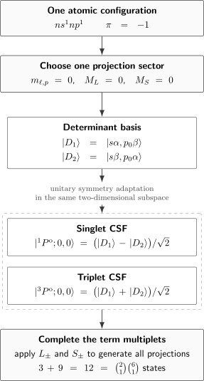
Within the $M_L=M_S=0$ sector of $ns^1np^1$, the determinant basis and the $LS$-adapted CSF basis span the same two-dimensional space. Relative signs shown here follow the spin-orbital ordering stated in the text; another consistent determinant convention can change displayed coefficient signs without changing the singlet and triplet subspaces.

Spatial and spin factorization

In coordinate space, the two combinations factor as

$$\begin{aligned} {}^1P^{\mathrm o}:\quad &\frac{s(1)p(2)+p(1)s(2)}{\sqrt2}\\ &\times \frac{\alpha(1)\beta(2)-\beta(1)\alpha(2)} {\sqrt2}, \end{aligned}$$

and

$$\begin{aligned} {}^3P^{\mathrm o}:\quad &\frac{s(1)p(2)-p(1)s(2)}{\sqrt2}\\ &\times \frac{\alpha(1)\beta(2)+\beta(1)\alpha(2)} {\sqrt2}. \end{aligned}$$

The total wavefunction is antisymmetric in both cases. The singlet uses a symmetric spatial factor and antisymmetric spin factor; the triplet uses the opposite pairing.

Completing the multiplets

The singlet $P$ term has

$$(2L+1)(2S+1)=3$$

magnetic states. The triplet $P$ term has

$$(2L+1)(2S+1)=9.$$

Together they account for all

$$3+9=12$$

determinants of the $ns^1np^1$ configuration. Ladder operators generate the other $M_L$ and $M_S$ components.

The exchange splitting between the two fixed-orbital spatial symmetries is developed at Exchange and Correlation. The present example concerns basis construction, not an energetic ordering rule.

Equivalent Electrons

For non-equivalent electrons, ordinary angular-momentum coupling and total antisymmetrization generate the expected $L$ and $S$ possibilities. Equivalent electrons occupy the same $n\ell$ subshell, so antisymmetry removes some naively coupled terms.

For $p^2$, the determinant space has dimension $15$, but only

$${}^1S,\qquad {}^3P,\qquad {}^1D$$

survive. Their magnetic dimensions satisfy

$$1+9+5=15.$$

This result is quoted here only to locate the determinant-to-CSF step. Its exchange-parity derivation, particle–hole relation, and shell-capacity consequences are canonical in Pauli Principle in Atoms.

For configurations with several equivalent open subshells, the same $LS$ term can occur more than once. Parent terms, seniority, quasispin, or another label may be needed to distinguish independent CSFs.

Determinants, CSFs, and Atomic Eigenstates

These objects form four distinct layers:

$$\begin{aligned} \text{configuration} &\longrightarrow \{|D\rangle\}\\ &\longrightarrow \{|\Phi_{\alpha\Gamma}\rangle\}\\ &\longrightarrow \{|\Psi_{k\Gamma}\rangle\}. \end{aligned}$$

1. A configuration fixes subshell populations.
2. A determinant fixes occupied complete spin-orbitals.
3. A CSF combines determinants to carry declared exact symmetries.
4. An approximate atomic eigenstate combines CSFs after the Hamiltonian is diagonalized.

For fixed symmetry $\Gamma$,

$$|\Psi_{k\Gamma}\rangle = \sum_{\alpha,I} c_{\alpha I}^{(k\Gamma)} |\Phi_{\alpha I\Gamma}\rangle.$$

The index $I$ can run over several configurations. Combining determinants within one configuration to obtain good symmetry is symmetry adaptation. Combining CSFs from different configurations to approximate an eigenstate is configuration interaction. Both are linear combinations, but they answer different questions.

A CSF is not automatically correlated

A multi-determinant CSF may be required solely because one determinant does not transform irreducibly under rotations and spin. Calling every such linear combination “electron correlation” obscures the distinction between exact symmetry adaptation and dynamical improvement of the wavefunction.

Conversely, a single determinant can contain exchange exactly while still missing correlation beyond its occupied subspace. Exchange and Correlation owns that accounting.

A configuration is not a level

Several terms can arise from one configuration, and several configurations can contribute to one level. A spectroscopic label usually records dominant ancestry and exact symmetry, not an assertion that one configuration or determinant is the complete state.

Relation to Hartree–Fock

Standard Hartree–Fock varies one determinant. A closed-shell atomic determinant is already adapted to $L=S=0$. An open-shell determinant can instead have only $M_L$ and $M_S$, or can deliberately break spin or spatial symmetry.

Atomic calculations use several related strategies:

• optimize one determinant and accept its symmetry content;
• constrain a restricted-open-shell determinant;
• optimize a spherical average over determinants;
• optimize a term-dependent CSF;
• optimize several CSFs simultaneously in a multiconfiguration self-consistent-field method.

The last two options may retain Hartree–Fock-like radial equations but are not literally the same variational family as unrestricted optimization over one determinant. Hartree–Fock for Atoms develops these distinctions and their orbital-energy consequences.

Orbital rotations

A unitary rotation among all occupied spin-orbitals of one determinant changes it only by the phase $\det U$. Its occupied subspace, density projector, and energy are unchanged.

A rotation that mixes occupied and unoccupied orbitals changes the determinant. More generally, rotating the one-electron basis can redistribute coefficients across determinants and configurations in a multi-CSF expansion. Exact symmetry labels and observables remain invariant; individual configuration percentages need not.

One- and Two-Electron Matrix Elements

Atomic Hamiltonians are dominated by one- and two-electron operators:

$$H = \sum_{pq}h_{pq}a_p^\dagger a_q +\frac14\sum_{pqrs} \langle pq\Vert rs\rangle a_p^\dagger a_q^\dagger a_s a_r.$$

The antisymmetrized two-electron integral is

$$\langle pq\Vert rs\rangle = \langle pq|v|rs\rangle -\langle pq|v|sr\rangle.$$

Fermionic anticommutation gives the Slater–Condon connectivity rules:

• a one-electron operator connects determinants that differ by at most one occupied spin-orbital;
• a two-electron operator connects determinants that differ by at most two occupied spin-orbitals;
• determinants differing by three or more occupations have zero matrix element for a one-plus-two-electron Hamiltonian.

For one determinant, the diagonal energy is

$$\begin{aligned} \langle D|H|D\rangle ={}& \sum_{i\in\mathrm{occ}}h_{ii}\\ &+\frac12 \sum_{i,j\in\mathrm{occ}} \langle ij\Vert ij\rangle. \end{aligned}$$

The sign of an off-diagonal determinant matrix element also contains the parity needed to reorder creation operators into the canonical sequence. This is why phase bookkeeping cannot be postponed until the end.

The connectivity rules make determinant Hamiltonian matrices sparse. Transforming to CSFs reduces them further into symmetry blocks and removes couplings forbidden by total angular momentum, spin, or parity.

One-Body Operators and Two-Body Operators own the general second-quantized derivations.

From LS CSFs to Fine-Structure Levels

In a purely electrostatic nonrelativistic Hamiltonian,

$$[H,L^2]=[H,S^2]=0,$$

so an $LS$-adapted basis block diagonalizes the Hamiltonian by $L$, $S$, and parity.

Spin-orbit and other relativistic interactions generally preserve total $J$ and parity but can mix CSFs with different $L$ and $S$:

$$|\Psi_{\gamma JM}^{\pi}\rangle = \sum_{\alpha LS} c_{\alpha LS}^{(\gamma J)} |\alpha LSJM;\pi\rangle.$$

The $LS$ labels then describe basis ancestry rather than exact quantum numbers. A relativistic $jj$-coupled CSF basis reaches the same physical $J^\pi$ sector through a different coupling order.

Atomic Term Symbols explains how configuration, term, level, and state labels are reported. Angular Momentum Coupling Schemes develops the change between $LS$, $jj$, and intermediate-coupling descriptions.

Practical Construction Workflow

1. Declare the one-electron basis. State whether orbitals are nonrelativistic $n\ell m_\ell m_s$ functions, relativistic spinors, real orbitals, numerical orbitals, or another basis.
2. Fix a canonical ordering. Every determinant and off-diagonal sign depends on it.
3. Specify the configuration or active space. List allowed subshell occupations and frozen-core assumptions.
4. Enumerate Pauli-allowed determinants. Do not assign particle identities.
5. Compute immediate labels. In an appropriate basis, record $M_L$, $M_S$, $M_J$, and parity.
6. Adapt to exact symmetries. Construct CSFs for the Hamiltonian’s commuting operators.
7. Check state counts. Determinant and CSF dimensions must agree.
8. Build Hamiltonian blocks. Use one- and two-body connectivity plus angular selection rules.
9. Diagonalize and interpret. Distinguish basis coefficients from exact symmetry labels and observables.
10. Document conventions. Record orbital ordering, coupling tree, phase convention, and normalization.

Common Mistakes

“A configuration is a determinant”

A configuration fixes subshell populations. An open-shell configuration usually generates many determinants with different occupied $m_\ell,m_s$ modes.

“A determinant has a term symbol”

A determinant in an $m_\ell,m_s$ basis has projection labels and parity. It generally contains several $L,S$ components. A term symbol belongs to a symmetry-adapted state.

“Every CSF is one determinant”

Closed shells and some stretched components can be represented by one determinant. Generic open-shell CSFs require linear combinations.

“Any multi-determinant expression is correlation”

Several determinants may be required simply to construct an eigenstate of $L^2$ and $S^2$. Correlation is a separate statement about improving the physical state beyond a declared reference.

“Opposite-spin electrons are distinguishable”

The complete determinant is antisymmetric under exchange of any two electron spin-space coordinates. Orthogonal spin functions can make an exchange matrix element vanish without changing particle identity.

“Changing determinant order changes the physics”

An odd reordering changes a determinant’s sign. One overall sign is conventional, but inconsistent relative signs corrupt CSFs and matrix elements.

“Spherical orbitals guarantee a good L”

Individual $Y_{\ell m}$ orbitals have definite $\ell,m$, but their determinant generally has only definite $M_L$. Total $L$ requires coupling.

“A configuration percentage is an observable”

Configuration weights depend on the orbital basis, coupling convention, and retained model space. They are useful diagnostics only with those choices stated.

Exercises

Exercise 1: Count atomic determinants

Count the determinants generated by $np^2$, $ns^1np^1$, and a closed $np^6$ subshell.

Solution

An $s$ subshell has capacity $2$, while a $p$ subshell has capacity $6$. Therefore

$$\begin{aligned} \dim\mathcal D(np^2) &=\binom62=15,\\ \dim\mathcal D(ns^1np^1) &=\binom21\binom61=12,\\ \dim\mathcal D(np^6) &=\binom66=1. \end{aligned}$$

The counts precede symmetry adaptation. The unique closed-subshell determinant is a scalar, while the open-shell determinant spaces decompose into several magnetic components and terms.

Exercise 2: Read determinant quantum numbers

In a complex $p$-orbital basis, consider a determinant containing $p_{m=1}\alpha$ and $p_{m=0}\beta$. Find $M_L$, $M_S$, and parity. Does this identify one term?

Solution

The projections are

$$\begin{aligned} M_L&=1+0=1,\\ M_S&=\frac12-\frac12=0. \end{aligned}$$

Each $p$ orbital has odd one-electron parity, so the two-electron determinant has

$$\pi=(-1)^{1+1}=+1.$$

These labels do not identify one term. For equivalent $p^2$ electrons, the determinant can have components in allowed even-parity terms compatible with $M_L=1$ and $M_S=0$. One must project or combine determinants to obtain definite $L$ and $S$.

Exercise 3: Track a determinant sign

Let $p<q<r$ be the canonical spin-orbital order. Rewrite

$$a_r^\dagger a_p^\dagger a_q^\dagger|0\rangle$$

in canonical order.

Solution

Move $a_r^\dagger$ past $a_p^\dagger$ and then past $a_q^\dagger$. Two fermionic swaps give

$$\begin{aligned} a_r^\dagger a_p^\dagger a_q^\dagger &= -a_p^\dagger a_r^\dagger a_q^\dagger\\ &= +a_p^\dagger a_q^\dagger a_r^\dagger. \end{aligned}$$

The permutation is even, so the canonical determinant has a plus sign.

Exercise 4: Spin-adapt the s-p sector

Using the determinant convention in the worked example, show that

$$\frac{|D_1\rangle-|D_2\rangle}{\sqrt2}$$

is a singlet and the orthogonal plus combination is a triplet component.

Solution

The spin-raising operator changes a $\beta$ occupation into the corresponding $\alpha$ occupation. With the declared canonical order, both determinants are raised to the same $M_S=1$ determinant with the same sign:

$$\begin{aligned} S_+|D_1\rangle &=\hbar|s\alpha,p_0\alpha\rangle,\\ S_+|D_2\rangle &=\hbar|s\alpha,p_0\alpha\rangle. \end{aligned}$$

Therefore

$$S_+ \frac{|D_1\rangle-|D_2\rangle}{\sqrt2} =0.$$

At $M_S=0$, a state annihilated by $S_+$ has $S=0$. The plus combination is raised to a nonzero $M_S=1$ state and belongs to $S=1$. Since one $s$ and one $p$ electron can only have $L=1$, the two CSFs are $^{1}P^{\mathrm o}$ and $^{3}P^{\mathrm o}$.

Exercise 5: Close the s-p state count

Verify that the $^{1}P^{\mathrm o}$ and $^{3}P^{\mathrm o}$ terms exhaust the determinant space of $ns^1np^1$.

Solution

The singlet term has

$$(2L+1)(2S+1) = 3\times1=3$$

magnetic states. The triplet term has

$$(2L+1)(2S+1) = 3\times3=9.$$

Their sum is

$$3+9=12,$$

which equals $\binom21\binom61$. No determinant states remain unassigned and none are counted twice.

Exercise 6: Apply the connectivity rule

For a Hamiltonian containing only one- and two-electron operators, decide whether two determinants can have a nonzero matrix element if they differ in zero, one, two, or three occupied spin-orbitals.

Solution

Identical determinants have diagonal matrix elements. Determinants differing by one occupation can be connected by the one-electron operator and also by parts of the two-electron operator involving shared spectators. Determinants differing by two occupations can be connected by the two-electron operator.

If three or more occupied spin-orbitals differ, neither a one-body operator nor a two-body operator can transform one occupation pattern into the other. The matrix element vanishes.

Exercise 7: Name the four layers

An atomic calculation starts from $2s^2\,2p^2$, constructs 15 open-subshell occupation patterns, combines them into even-parity $^{1}S$, $^{3}P$, and $^{1}D$ functions, then mixes the $^{1}S$ function with a $2s^2\,2p^0\,3s^2$ function of the same symmetry. Identify the configuration, determinant, CSF, and eigenstate layers.

Solution

$2s^2\,2p^2$ and $2s^2\,3s^2$ are configurations because they state subshell populations. Each of the 15 allowed $2p^2$ spin-orbital occupation patterns is a determinant when placed in the declared orbital order.

The $^{1}S$, $^{3}P$, and $^{1}D$ functions are CSFs obtained by symmetry-adapting determinants within the first configuration. The final $^{1}S$ eigenvector is a configuration-interaction combination of at least two $^{1}S$ CSFs from different configurations.

The first linear combination enforces symmetry. The second uses Hamiltonian mixing to improve a state with that symmetry.

Key Takeaways

• An atomic determinant occupies complete spin-orbitals and is antisymmetric by construction.
• In an $m_\ell,m_s$ basis, a determinant has definite $M_L$, $M_S$, and parity, but generally not definite $L$ or $S$.
• A configuration fixes subshell populations; one open-shell configuration usually generates many determinants.
• A CSF is a symmetry-adapted determinant combination with declared $LS\pi$ or $J^\pi$ labels.
• Determinant and CSF bases span the same declared antisymmetric space when both are complete.
• State-count closure tests whether every determinant has been assigned to exactly one coupled multiplet component.
• Relative determinant signs depend on orbital ordering and angular-momentum conventions and must be handled consistently.
• Symmetry adaptation within a configuration is distinct from configuration interaction across configurations.
• One- and two-electron Hamiltonians connect determinants differing by at most two occupations.
• Hartree–Fock, open-shell averages, term-dependent optimization, and multiconfiguration methods use related but different determinant or CSF variational spaces.

Cross-Links

• Multi-Electron Atoms
• Electron Configurations
• Pauli Principle in Atoms
• Exchange and Correlation
• Hartree–Fock for Atoms
• LS Coupling
• Helium Atom
• Atomic Orbitals Revisited
• Atomic Term Symbols
• Atomic Selection Rules
• Slater Determinants
• Spin and Spatial Wavefunctions
• Occupation-Number Basis
• Creation and Annihilation Operators
• Fermionic Anticommutation Relations
• One-Body Operators
• Two-Body Operators
• Clebsch–Gordan Coefficients
• Clebsch–Gordan Tables and Conventions
• Angular Momentum Coupling Schemes

References

• J. C. Slater, “The Theory of Complex Spectra,” Physical Review 34, 1293–1322 (1929), doi:10.1103/PhysRev.34.1293.
• E. U. Condon and G. H. Shortley, The Theory of Atomic Spectra, Cambridge University Press (1935).
• G. Racah, “Theory of Complex Spectra. II,” Physical Review 62, 438–462 (1942), doi:10.1103/PhysRev.62.438.
• R. D. Cowan, The Theory of Atomic Structure and Spectra, University of California Press (1981).
• B. R. Judd, Operator Techniques in Atomic Spectroscopy, McGraw–Hill (1963).
• C. Froese Fischer, T. Brage, and P. Jönsson, Computational Atomic Structure: An MCHF Approach, Institute of Physics Publishing (1997).
• I. P. Grant, Relativistic Quantum Theory of Atoms and Molecules: Theory and Computation, Springer (2007).
• A. Szabo and N. S. Ostlund, Modern Quantum Chemistry: Introduction to Advanced Electronic Structure Theory, Dover (1996).
• R. McWeeny, Methods of Molecular Quantum Mechanics, 2nd ed., Academic Press (1992).
• A. R. Edmonds, Angular Momentum in Quantum Mechanics, Princeton University Press (1957).