Rabi Formula in the Weak-Drive Limit

The Rabi formula and first-order time-dependent perturbation theory describe the same driven two-level system in an overlap regime, but they organize the physics differently. The Rabi formula resums repeated transitions and preserves bounded population dynamics. First-order theory keeps only the leading transition amplitude and is simpler, more general, and directly connected to the Fourier spectrum of a weak pulse.

This page owns the asymptotic match between those descriptions. The exact model and its Bloch-sphere interpretation live in Rabi Oscillations: First Encounter. Resonant Driving owns finite-pulse linewidths and resonance-regime diagnostics, while the Rotating-Wave Approximation owns the removal of counter-rotating terms.

Model and Conventions

Assume an isolated two-level subspace with lower state $\lvert g\rangle$, upper state $\lvert e\rangle$, and bare transition angular frequency $\omega_0$. A monochromatic drive at angular frequency $\omega$ is reduced, after a rotating-frame transformation and the rotating-wave approximation, to

$$H_{\mathrm{eff}} = \frac{\hbar}{2} \left( \Delta\sigma_z + \Omega\sigma_x \right),$$

where

$$\Delta = \omega_0-\omega$$

is the detuning and $\Omega$ is the on-resonance Rabi angular frequency in this convention. The factor of $1/2$ in the Hamiltonian matters: other conventions can differ by a factor of two in the symbol called the Rabi frequency.

Choose

$$\sigma_z\lvert e\rangle = \lvert e\rangle, \qquad \sigma_z\lvert g\rangle = -\lvert g\rangle.$$

The generalized Rabi angular frequency is

$$\Omega_R = \sqrt{\Omega^2+\Delta^2}.$$

For a square pulse of duration $T$ and initial state $\lvert g\rangle$, the exact transition probability within this effective model is

$$P_{\mathrm{R}}(T) = \frac{\Omega^2}{\Omega_R^2} \sin^2\left( \frac{\Omega_RT}{2} \right).$$

“Exact” here means exact for the time-independent two-level effective Hamiltonian. It does not undo errors from truncating other levels, making the rotating-wave approximation, neglecting dissipation, or idealizing the pulse as rectangular.

Exact Evolution Operator

The Pauli identity

$$\left( \Delta\sigma_z+ \Omega\sigma_x \right)^2 = \Omega_R^2 I$$

lets the exponential be evaluated directly:

$$U_{\mathrm{eff}}(T) = \exp\left( -\frac{i}{\hbar}H_{\mathrm{eff}}T \right).$$

Define the unit-axis operator

$$N \equiv \frac{ \Delta\sigma_z+\Omega\sigma_x }{\Omega_R}, \qquad N^2=I.$$

Then

$$\begin{aligned} U_{\mathrm{eff}}(T) &= \cos\left( \frac{\Omega_RT}{2} \right)I \\ &\quad -iN \sin\left( \frac{\Omega_RT}{2} \right). \end{aligned}$$

The rotating-frame excited-state amplitude is therefore

$$b_e(T) = -i\frac{\Omega}{\Omega_R} \sin\left( \frac{\Omega_RT}{2} \right).$$

Transforming back to the interaction-picture coefficient used in transition theory supplies a convention-dependent phase. With the choices above,

$$c_e(T) = -i e^{i\Delta T/2} \frac{\Omega}{\Omega_R} \sin\left( \frac{\Omega_RT}{2} \right).$$

The phase cancels from the population but matters in Ramsey sequences, coherent pathway interference, and state tomography.

First-Order Transition Result

In the interaction picture, the retained rotating term is

$$V_I^{\mathrm{RWA}}(t) = \frac{\hbar\Omega}{2} \left( \sigma_+e^{i\Delta t} + \sigma_-e^{-i\Delta t} \right).$$

Starting from $\lvert g\rangle$, first order gives

$$\begin{aligned} c_e^{(1)}(T) &= -\frac{i\Omega}{2} \int_0^Tdt\,e^{i\Delta t} \\ &= -i e^{i\Delta T/2} \frac{\Omega T}{2} \operatorname{sinc} \left( \frac{\Delta T}{2} \right). \end{aligned}$$

Thus

$$P_{\mathrm{PT}}(T) = \frac{\Omega^2T^2}{4} \operatorname{sinc}^2 \left( \frac{\Delta T}{2} \right).$$

This is the leading probability obtained by squaring the first-order amplitude. It is second order in the drive strength even though it is conventionally called a first-order perturbation-theory result.

Dimensionless Matching Variables

Introduce

$$a \equiv \Omega T, \qquad d \equiv \Delta T.$$

The exact Rabi probability becomes

$$P_{\mathrm{R}}(a,d) = \frac{a^2}{a^2+d^2} \sin^2\left[ \frac{1}{2} \sqrt{a^2+d^2} \right],$$

whereas first-order transition theory gives

$$P_{\mathrm{PT}}(a,d) = \frac{a^2}{4} \operatorname{sinc}^2 \left( \frac{d}{2} \right).$$

These variables expose the two competing accumulated phases:

• $a=\Omega T$ is the pulse area for a constant real coupling;
• $d=\Delta T$ is the detuning phase accumulated during the pulse.

Weak instantaneous coupling is not enough. The expansion that connects the formulas is an expansion in $a$ at fixed $d$, or an off-resonant expansion in $\Omega/\lvert\Delta\rvert$ with its own long-time caveats.

Leading Weak-Drive Expansion

For fixed $d\ne0$ and $a\to0$,

$$\sqrt{a^2+d^2} = \lvert d\rvert \left[ 1+ \frac{a^2}{2d^2} +O\!\left( \frac{a^4}{d^4} \right) \right].$$

At leading order,

$$\begin{aligned} P_{\mathrm{R}}(a,d) &= \frac{a^2}{d^2} \sin^2\left( \frac{d}{2} \right) +O(a^4) \\ &= \frac{a^2}{4} \operatorname{sinc}^2\left( \frac{d}{2} \right) +O(a^4). \end{aligned}$$

Therefore

$$P_{\mathrm{R}}(a,d) = P_{\mathrm{PT}}(a,d) +O(a^4)$$

at fixed $d$. At the amplitude level,

$$c_e(a,d) = c_e^{(1)}(a,d) +O(a^3).$$

The next correction to the amplitude is third order because each interaction flips the two-level state: an odd number of flips is required to end in $\lvert e\rangle$. The probability correction begins at fourth order through interference between the first- and third-order amplitudes.

First Correction and Error Structure

Expanding one order further gives

$$P_{\mathrm{R}}(a,d) = P_{\mathrm{PT}}(a,d) +a^4 C(d) +O(a^6),$$

where

$$C(d) = \frac{ \tfrac14 d\sin d - \sin^2(d/2) }{d^4}.$$

Although this expression appears singular at $d=0$, the singularity is removable. Series expansion gives

$$C(0) = -\frac{1}{48}.$$

At a zero of the leading sinc profile, a relative error based on $P_{\mathrm{PT}}$ is not useful because the denominator vanishes. There the correct diagnostic is absolute error or the first nonzero higher-order transition amplitude.

For a requested tolerance, one should compare the actual observable rather than invoke “weak drive” qualitatively. At fixed $d$ away from a leading zero, the relative population error generally scales as $a^2$.

Exact Resonance

Setting $d=0$ gives

$$P_{\mathrm{R}}(a,0) = \sin^2\left( \frac{a}{2} \right),$$

while

$$P_{\mathrm{PT}}(a,0) = \frac{a^2}{4}.$$

Their expansions agree initially:

$$\begin{aligned} P_{\mathrm{R}}(a,0) &= \frac{a^2}{4} - \frac{a^4}{48} +O(a^6), \\ P_{\mathrm{PT}}(a,0) &= \frac{a^2}{4}. \end{aligned}$$

The relative overestimate from first order is

$$\frac{ P_{\mathrm{PT}}-P_{\mathrm{R}} }{P_{\mathrm{R}}} = \frac{a^2}{12} +O(a^4).$$

Some representative values are:

Pulse area $a$	Exact $\sin^2(a/2)$	First order $a^2/4$	Relative overestimate
$0.1$	$0.00249792$	$0.00250000$	$0.083\%$
$0.5$	$0.06120872$	$0.06250000$	$2.110\%$
$1$	$0.22984885$	$0.25000000$	$8.767\%$
$\pi$	$1$	$2.46740110$	$146.740\%$

The $\pi$-pulse row makes the failure unmistakable. A pulse can be weak relative to the carrier frequency and still have order-one area because it acts for a long time.

Far-Off-Resonant Limit

When

$$\lvert\Delta\rvert \gg \lvert\Omega\rvert,$$

the exact maximum population obeys

$$P_{e,\max} = \frac{\Omega^2}{\Omega^2+\Delta^2} \simeq \frac{\Omega^2}{\Delta^2}.$$

Population transfer can therefore remain perturbatively small for times much longer than $1/\Omega$. However, the generalized frequency contains the shift

$$\Omega_R = \lvert\Delta\rvert + \frac{\Omega^2}{2\lvert\Delta\rvert} + O\!\left( \frac{\Omega^4}{\lvert\Delta\rvert^3} \right).$$

The second-order frequency correction accumulates a substantial phase on the scale

$$T_{\mathrm{shift}} \sim \frac{\lvert\Delta\rvert}{\Omega^2}.$$

Thus “the transition probability stays small” and “the full state is accurately described to first order” are different claims. Off-resonant drives can produce important phases and effective energy shifts without transferring much population.

The Weak and Long-Time Limits Do Not Commute

At fixed $T$,

$$\Omega\to0$$

implies $a\to0$, and first-order theory becomes accurate. But consider a family of resonant pulses with

$$T_\Omega = \frac{\pi}{\Omega}.$$

As $\Omega\to0$, the instantaneous drive becomes arbitrarily weak while the pulse area remains

$$\Omega T_\Omega = \pi.$$

For every member of the family,

$$P_{\mathrm{R}} = 1,$$

whereas first order predicts

$$P_{\mathrm{PT}} = \frac{\pi^2}{4} \gt 1.$$

This is a singular long-time scaling limit. Statements about weak drive must specify what is held fixed as the drive strength decreases.

Three Independent Approximations

The standard Rabi formula often sits behind several layers of approximation. Their control parameters are not interchangeable.

Step	What is neglected?	Typical diagnostic	Can it hold while first order fails?
Two-level reduction	Other states and leakage pathways	spectral gaps and unwanted matrix elements	Yes; an isolated resonant pair can undergo full Rabi cycles
Rotating-wave approximation	Counter-rotating terms	$\lvert\Omega\rvert,\lvert\Delta\rvert\ll\omega_0+\omega$ plus envelope slowness	Yes; a long resonant $\pi$ pulse can satisfy the RWA very well
First-order transition theory	Repeated transitions and depletion	$\lvert c_e^{(1)}\rvert\ll1$, or $a\ll1$ near resonance	No; this row is the condition being tested
Closed-system description	Relaxation, dephasing, measurement backaction	$T\ll T_1,T_2$ for coherent pulsed dynamics	Yes; unitary Rabi cycling can be nonperturbative

The converse separations also matter. A very short, broadband pulse can produce only a small transition probability while invalidating a narrowband rotating-wave treatment. A far-detuned weak drive can leave populations perturbative while generating a measurable second-order phase.

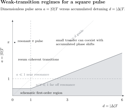
For a square pulse, the natural coordinates are $a=\lvert\Omega\rvert T$ and $d=\lvert\Delta\rvert T$. Near resonance, first-order transition theory requires $a\ll1$; far off resonance, small population transfer follows from $a/d=\lvert\Omega/\Delta\rvert\ll1$. The shaded region is schematic rather than a universal error contour. RWA validity depends additionally on the unshown fast scale $\omega_0+\omega$.

General Pulse Envelope

Let the rotating-wave interaction contain a complex, time-dependent coupling $\Omega(t)$:

$$\begin{aligned} V_I^{\mathrm{RWA}}(t) &= \frac{\hbar}{2} \big[ \Omega(t)e^{i\Delta t}\sigma_+ \\ &\qquad +\Omega^*(t)e^{-i\Delta t}\sigma_- \big]. \end{aligned}$$

First order gives the general weak-pulse amplitude

$$c_e^{(1)} = -\frac{i}{2} \int_{t_0}^{t_1}dt\, \Omega(t)e^{i\Delta t}.$$

Define

$$\eta \equiv \frac{1}{2} \left\lvert \int_{t_0}^{t_1}dt\, \Omega(t)e^{i\Delta t} \right\rvert.$$

Then the leading population is

$$P_e^{(1)} = \eta^2,$$

and a transition-specific perturbative condition is

$$\eta \ll 1.$$

The triangle inequality gives the conservative sufficient condition

$$\eta \le \frac{1}{2} \int_{t_0}^{t_1}dt\, \lvert\Omega(t)\rvert \ll 1.$$

This stronger condition ignores detuning cancellations. It is useful for guaranteed bounds but can be far more restrictive than necessary for an off-resonant pulse.

On exact resonance with fixed drive phase, all effective Hamiltonians point along the same Bloch-sphere axis, and the full result depends on pulse area. Once detuning, chirp, or phase modulation changes that axis, time ordering matters and pulse area alone is insufficient.

Amplitude Accuracy Versus Population Accuracy

A small population error does not guarantee a small phase error. Suppose

$$c_e = c_e^{(1)} + c_e^{(3)} + \cdots.$$

Then

$$\begin{aligned} P_e &= \lvert c_e^{(1)}\rvert^2 \\ &\quad +2\operatorname{Re} \left[ c_e^{(1)*}c_e^{(3)} \right] +O(\Omega^6). \end{aligned}$$

The leading probability can be accurate even when a small higher-order phase matters to an interferometric observable. Conversely, near a zero of $c_e^{(1)}$, a higher-order amplitude can control the entire nonzero signal even though its absolute magnitude is tiny.

A validity statement should therefore name the target observable: population, complex amplitude, phase, line center, or time-resolved trajectory.

Multilevel Extension

For several possible final states, the first-order amplitudes take the form

$$c_f^{(1)} = -\frac{i}{\hbar} \int_{t_0}^{t_1}dt\, e^{i\omega_{fi}t}V_{fi}(t).$$

A basic depletion diagnostic is

$$\sum_{f\ne i} \lvert c_f^{(1)}\rvert^2 \ll 1$$

for discrete states, with the sum replaced by the appropriate continuum integral when needed. If a set of states is mutually near resonant, that subspace should be retained and solved nonperturbatively rather than forcing independent two-level formulas onto overlapping lines.

The two-level Rabi formula also misses leakage, dark and bright superpositions, Raman pathways, and multiphoton processes. Those effects require the actual coupling graph and the relevant order of the Dyson Expansion for Transition Amplitudes.

Choosing the Description

Goal or regime	Appropriate starting point
Small population after a specified weak pulse	First-order transition amplitude
Coherent inversion or repeated population exchange	Exact or numerically solved few-level Hamiltonian
Weak near-resonant monochromatic drive with counter-rotating separation	Rotating-wave effective Hamiltonian
Precision line center or long off-resonant phase	Include higher-order shifts and counter-rotating corrections
Decay into a smooth continuum	Fermi’s golden rule within its time window
Relaxation, dephasing, saturation, or steady state	Optical Bloch or another open-system equation
Strong periodic drive outside the RWA	Floquet or direct time-dependent evolution

The formulas are not competitors. They answer different questions at different resolutions.

Common Mistakes

• Calling the Rabi formula universally exact. It is exact only for the chosen effective two-level Hamiltonian.
• Expanding in $\Omega$ while silently letting $T$ scale as $1/\Omega$. The accumulated parameter $a=\Omega T$ then remains order one.
• Using RWA validity as proof of first-order validity. The RWA can remain excellent through many nonperturbative Rabi cycles.
• Comparing formulas with different Rabi-frequency conventions. The Hamiltonian fixes whether a factor of two belongs in $\Omega$.
• Checking probability but ignoring phase. Off-resonant second-order shifts can dominate precision observables.
• Using relative error at a leading-order zero. Use absolute error or identify the first nonzero order instead.
• Forgetting other levels. A clean two-level match says nothing about leakage if the two-level reduction itself is invalid.
• Treating coherent oscillation as an irreversible rate. A closed discrete two-level system does not obey a constant golden-rule transition rate at all times.

Exercises

Derive the exact propagator

Starting from

$$H_{\mathrm{eff}} = \frac{\hbar}{2} \left( \Delta\sigma_z+\Omega\sigma_x \right),$$

derive $U_{\mathrm{eff}}(T)$ and the transition probability from $\lvert g\rangle$ to $\lvert e\rangle$.

Solution

Let

$$M = \Delta\sigma_z+\Omega\sigma_x.$$

The Pauli anticommutation relations give

$$M^2 = \left( \Delta^2+\Omega^2 \right)I = \Omega_R^2I.$$

Even powers of $M$ are proportional to $I$ and odd powers to $M$. Separating the exponential series gives

$$\begin{aligned} U_{\mathrm{eff}}(T) &= I\cos\left( \frac{\Omega_RT}{2} \right) \\ &\quad -i\frac{M}{\Omega_R} \sin\left( \frac{\Omega_RT}{2} \right). \end{aligned}$$

Because $\langle e\rvert\sigma_z\lvert g\rangle=0$ and $\langle e\rvert\sigma_x\lvert g\rangle=1$,

$$\langle e\rvert U_{\mathrm{eff}}(T)\lvert g\rangle = -i\frac{\Omega}{\Omega_R} \sin\left( \frac{\Omega_RT}{2} \right).$$

Taking the squared magnitude gives

$$P_e(T) = \frac{\Omega^2}{\Omega_R^2} \sin^2\left( \frac{\Omega_RT}{2} \right).$$

Compute the first correction

At fixed $d\ne0$, expand

$$P_{\mathrm{R}}(a,d) = \frac{a^2}{a^2+d^2} \sin^2\left[ \frac12\sqrt{a^2+d^2} \right]$$

through order $a^4$. Show that $C(d)$ has the finite limit $-1/48$ as $d\to0$.

Solution

Use

$$\frac{a^2}{a^2+d^2} = \frac{a^2}{d^2} \left( 1- \frac{a^2}{d^2} +O(a^4) \right)$$

and

$$\sqrt{a^2+d^2} = d+ \frac{a^2}{2d} +O(a^4)$$

for positive $d$; the final expression is even in $d$. Then

$$\begin{aligned} \sin^2\left[ \frac12\sqrt{a^2+d^2} \right] &= \sin^2\left( \frac d2 \right) \\ &\quad +\frac{a^2}{4d}\sin d \\ &\quad +O(a^4). \end{aligned}$$

Multiplying gives

$$\begin{aligned} P_{\mathrm{R}} &= \frac{a^2}{d^2} \sin^2\left( \frac d2 \right) \\ &\quad +a^4C(d) +O(a^6), \\ C(d) &= \frac{\sin d}{4d^3} - \frac{\sin^2(d/2)}{d^4}. \end{aligned}$$

The bracket is $C(d)$. Expanding $d\sin d/4$ and $\sin^2(d/2)$ around zero cancels the apparent $d^{-2}$ terms and leaves

$$C(d) = -\frac{1}{48} +O(d^2).$$

Weak but nonperturbative pulse

Let $\Omega/\omega_0=10^{-4}$ and take exact resonance. Choose $T=\pi/\Omega$. Which approximations can remain valid, and why does first-order transition theory fail?

Solution

The small ratio $\Omega/\omega_0$ can make the rotating-wave approximation excellent if the envelope is also slow and other levels are isolated. The pulse area is nevertheless

$$a = \Omega T = \pi.$$

The exact effective two-level result is

$$P_e = \sin^2\left( \frac\pi2 \right) = 1,$$

whereas first order gives $\pi^2/4\gt1$. Thus two-level reduction and the RWA may remain controlled while the transition-amplitude truncation fails because repeated resonant transfers are order one.

Off-resonant phase time scale

Assume $\lvert\Delta\rvert\gg\lvert\Omega\rvert$. Expand $\Omega_R$ and estimate when the phase generated by the second-order frequency shift becomes order one.

Solution

The binomial expansion gives

$$\Omega_R = \lvert\Delta\rvert + \frac{\Omega^2}{2\lvert\Delta\rvert} + O\!\left( \frac{\Omega^4}{\lvert\Delta\rvert^3} \right).$$

The correction to the oscillation phase is of order

$$\delta\phi \sim \frac{\Omega^2T}{\lvert\Delta\rvert},$$

up to a convention-dependent factor of order one. It becomes important at

$$T \sim \frac{\lvert\Delta\rvert}{\Omega^2}.$$

At that time the excited-state population can still be only order $\Omega^2/\Delta^2$. Small leakage does not imply negligible phase evolution.

General-pulse bound

Show that

$$\eta = \frac12 \left\lvert \int_{t_0}^{t_1}dt\, \Omega(t)e^{i\Delta t} \right\rvert$$

obeys $\eta\le\frac12\int\lvert\Omega(t)\rvert dt$. Explain why the bound can be loose.

Solution

The triangle inequality gives

$$\begin{aligned} \eta &\le \frac12 \int_{t_0}^{t_1}dt\, \left\lvert \Omega(t)e^{i\Delta t} \right\rvert \\ &= \frac12 \int_{t_0}^{t_1}dt\, \lvert\Omega(t)\rvert. \end{aligned}$$

The bound discards all phase cancellation. For large detuning or a shaped pulse with destructive spectral interference, the Fourier component at $\Delta$ can be much smaller than the unsigned pulse area. The bound is sufficient for small transition amplitude but not necessary.

Choose the approximation

Classify the appropriate starting method in each case: (a) a resonant $\pi$ pulse in an isolated qubit, (b) a weak short pulse producing a $10^{-4}$ excitation probability, (c) continuous resonant driving with spontaneous emission for times much longer than $T_1$, and (d) a weak far-detuned drive used to accumulate a precision phase.

Solution

(a) Use exact or numerically solved two-level dynamics; first order cannot describe inversion.

(b) First-order transition theory is a natural starting point, provided leakage and bandwidth assumptions are checked.

(c) Use the optical Bloch equations or another open-system master equation. Closed Rabi dynamics omit relaxation and the steady state.

(d) Population transfer may be treated perturbatively, but the phase requires at least the second-order effective shift. A first-order population calculation alone is insufficient.

Cross-Links

• Rabi Oscillations: First Encounter
• Resonant Driving
• First-Order Transition Probability
• Harmonic Perturbations
• Rotating-Wave Approximation
• Rotating Frames
• Small Parameters and Error Estimates
• Dyson Expansion for Transition Amplitudes
• Fermi’s Golden Rule
• Optical Bloch Equations
• Two-Level System Reference

References

• I. I. Rabi, “Space Quantization in a Gyrating Magnetic Field,” Physical Review 51, 652–654, 1937.
• F. Bloch and A. Siegert, “Magnetic Resonance for Nonrotating Fields,” Physical Review 57, 522–527, 1940.
• L. Allen and J. H. Eberly, Optical Resonance and Two-Level Atoms, Dover, 1987.
• B. W. Shore, The Theory of Coherent Atomic Excitation, Wiley, 1990.
• C. Cohen-Tannoudji, J. Dupont-Roc, and G. Grynberg, Atom–Photon Interactions: Basic Processes and Applications, Wiley, 1992.
• J. J. Sakurai and J. Napolitano, Modern Quantum Mechanics, 3rd ed., Cambridge University Press, 2020.