Ehrenfest Theorem Overview

Ehrenfest theorem is an exact statement about the motion of quantum expectation values. For a standard particle Hamiltonian, the mean position and mean momentum obey equations that resemble Hamilton’s equations:

$$\frac{d}{dt}\langle x\rangle = \frac{\langle p\rangle}{m}, \qquad \frac{d}{dt}\langle p\rangle = \langle F(x)\rangle.$$

The resemblance contains the theorem’s value and its main trap. Classical mechanics would place the force at the classical position, $F(x_{\mathrm{cl}})$. Quantum mechanics gives the mean of the force, $\langle F(x)\rangle$. In general,

$$\langle F(x)\rangle \neq F(\langle x\rangle).$$

The theorem is therefore best read in two layers:

1. The expectation-value identity is exact whenever its analytic assumptions hold.
2. Classical centroid motion requires an additional closure approximation that replaces the mean force by the force at the mean.

This page develops that distinction and its physical use. The canonical operator derivation belongs to Ehrenfest Theorem; the full moment hierarchy and long-time analysis belong to Ehrenfest Theorem Revisited.

General Statement

For a normalized state evolving under $H(t)$ and an observable $A(t)$ with possible explicit time dependence,

$$\frac{d}{dt}\langle A\rangle = \frac{i}{\hbar} \langle[H,A]\rangle + \left\langle \frac{\partial A}{\partial t} \right\rangle.$$

Equivalently,

$$\frac{d}{dt}\langle A\rangle = \frac{1}{i\hbar} \langle[A,H]\rangle + \left\langle \frac{\partial A}{\partial t} \right\rangle.$$

The first term describes change generated by the Hamiltonian. The second accounts for explicit time dependence in the observable itself. For an operator with no explicit time dependence, only the commutator remains.

The same identity holds for a density operator:

$$\langle A\rangle = \operatorname{Tr}(\rho A),$$

provided the trace and derivative manipulations are justified. Thus Ehrenfest theorem applies to pure states, mixed preparations, and reduced states, not only to wave packets.

Analytic assumptions

For bounded operators in finite dimension, the formula is routine. Position, momentum, and most Hamiltonians in wave mechanics are unbounded, so a careful statement also requires:

• a differentiable state evolution;
• a state in the domains needed for $H$, $A$, and the relevant products;
• finite expectation values;
• boundary conditions that eliminate unintended surface terms;
• sufficient regularity to interchange differentiation, integration, and traces.

Introductory problems usually satisfy these conditions by construction. They become visible for singular potentials, hard boundaries, scattering states, and formal generalized eigenvectors.

Particle Form

Consider one spatial dimension with

$$H = \frac{p^2}{2m} + V(x),$$

where $x$ and $p$ have no explicit time dependence and

$$[x,p] = i\hbar.$$

The required commutators are

$$[H,x] = -\frac{i\hbar}{m}p$$

and

$$[H,p] = i\hbar V'(x).$$

Substitution into the general identity gives

$$\frac{d}{dt}\langle x\rangle = \frac{\langle p\rangle}{m}$$

and

$$\frac{d}{dt}\langle p\rangle = -\langle V'(x)\rangle.$$

Writing

$$F(x) = -V'(x),$$

the exact second-order equation is

$$m \frac{d^2}{dt^2} \langle x\rangle = \langle F(x)\rangle.$$

No narrow-packet, large-mass, or small-$\hbar$ approximation has entered. This exactness is sometimes obscured because the equation already looks Newtonian.

In several dimensions,

$$\frac{d}{dt} \langle\mathbf r\rangle = \frac{\langle\mathbf p\rangle}{m},$$

and

$$\frac{d}{dt} \langle\mathbf p\rangle = -\langle\nabla V(\mathbf r)\rangle.$$

The same closure issue then applies component by component.

Newton’s Law Is a Closure Condition

Let

$$\overline x = \langle x\rangle, \qquad \overline p = \langle p\rangle.$$

A classical trajectory initialized at $(\overline x,\overline p)$ would obey

$$m\ddot x_{\mathrm{cl}} = F(x_{\mathrm{cl}}).$$

The quantum centroid obeys

$$m\ddot{\overline x} = \langle F(x)\rangle.$$

Define the force-closure remainder

$$R_F = \langle F(x)\rangle - F(\overline x).$$

Then the exact centroid equation can be written as

$$m\ddot{\overline x} = F(\overline x) + R_F.$$

The centroid follows Newton’s equation when $R_F$ vanishes or remains negligible compared with the force accuracy required by the problem. Ehrenfest theorem supplies the exact left-hand side and exact mean force; it does not set $R_F$ to zero.

Exact Closure

The remainder vanishes for every state when the force is affine:

$$F(x) = f_0 + f_1x.$$

Linearity of expectation values then gives

$$\langle F(x)\rangle = f_0 + f_1\langle x\rangle = F(\overline x).$$

This includes potentials at most quadratic in position.

Potential	Force	Centroid motion
$V=V_0$	$F=0$	Free uniform motion
$V=-fx$	$F=f$	Constant acceleration
$V=\tfrac12m\omega^2x^2$	$F=-m\omega^2x$	Harmonic motion
General quadratic plus linear terms	Affine force	Exact classical linear equation

For the harmonic oscillator,

$$\ddot{\overline x} + \omega^2\overline x = 0$$

for every state for which the expectations exist. A coherent state, a number state, a squeezed state, and a separated superposition all have centroids satisfying this same equation.

That does not make their full probability distributions classically equivalent. Exact centroid closure is a statement about first moments only.

Approximate Closure for a Narrow Packet

Write

$$\delta x = x-\overline x, \qquad \mu_n = \langle(\delta x)^n\rangle.$$

Here $\mu_1=0$ and $\mu_2=\sigma_x^2$. Taylor expansion of the force gives

$$\begin{aligned} F(x) &= F(\overline x) + F'(\overline x)\delta x\\ &\quad+ \frac12 F''(\overline x)(\delta x)^2\\ &\quad+ \frac16 F'''(\overline x)(\delta x)^3 + \cdots. \end{aligned}$$

Taking the expectation value yields

$$\begin{aligned} \langle F(x)\rangle &= F(\overline x) + \frac12 F''(\overline x)\sigma_x^2\\ &\quad+ \frac16 F'''(\overline x)\mu_3 + \cdots. \end{aligned}$$

Therefore

$$R_F = \frac12 F''(\overline x)\sigma_x^2 + \frac16 F'''(\overline x)\mu_3 + \cdots.$$

For a nearly symmetric narrow packet, $\mu_3$ is small and the variance term is often the leading correction. A useful local criterion is

$$\frac{ \lvert F''(\overline x)\rvert \sigma_x^2 }{ 2F_* } \ll 1,$$

where $F_*$ is a force scale appropriate to the prediction. Near a force zero, using $\lvert F(\overline x)\rvert$ as the denominator is inappropriate; one must choose a nonzero experimental or dynamical scale.

The phrase “the packet is narrow” is thus relative to the curvature scale of the force and the desired accuracy, not an absolute statement about meters.

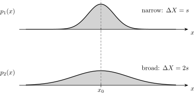
The same centroid does not imply the same mean force. When $F(x)$ is nonlinear, two states with common mean $x_0$ but different widths generally have different values of $\langle F(x)\rangle$.

Worked Example: Quartic Anharmonicity

Consider

$$V(x) = \frac12m\omega^2x^2 + \lambda x^4.$$

The force is

$$F(x) = -m\omega^2x - 4\lambda x^3.$$

Ehrenfest theorem gives

$$m\ddot{\overline x} = -m\omega^2\overline x - 4\lambda\langle x^3\rangle.$$

The third raw moment can be expressed through central moments:

$$\langle x^3\rangle = \overline x^3 + 3\overline x\,\sigma_x^2 + \mu_3.$$

Hence

$$\begin{aligned} m\ddot{\overline x} &= -m\omega^2\overline x - 4\lambda\overline x^3\\ &\quad- 12\lambda\overline x\,\sigma_x^2 - 4\lambda\mu_3. \end{aligned}$$

The first row is Newton’s equation evaluated at the centroid. The second row is the leading quantum-state correction. Even if the packet is initially symmetric so that $\mu_3=0$, its variance affects the centroid whenever $\overline x\neq0$.

This example exposes the closure problem cleanly: the first moment depends on second and third central moments. Their evolution can depend on still higher moments.

Width and Covariance Have Their Own Dynamics

Classical-looking centroid motion must persist, not merely hold at the initial time. Define

$$\delta p = p-\overline p$$

and the symmetrized covariance

$$C_{xp} = \frac12 \left\langle \delta x\,\delta p + \delta p\,\delta x \right\rangle.$$

The first second-moment equations are

$$\frac{d\sigma_x^2}{dt} = \frac{2}{m}C_{xp},$$ $$\frac{dC_{xp}}{dt} = \frac{\sigma_p^2}{m} - \langle\delta x\,V'(x)\rangle,$$

and

$$\frac{d\sigma_p^2}{dt} = -\left\langle \delta p\,V'(x) + V'(x)\,\delta p \right\rangle.$$

For a quadratic potential, this hierarchy closes among the first and second moments. For an anharmonic potential, new mixed and higher moments appear. That is why an initially narrow packet can spread, shear, or become multimodal, eventually invalidating

$$\langle F(x)\rangle \approx F(\overline x).$$

The detailed hierarchy, including uncertainty propagation and Ehrenfest-time estimates, is developed in Ehrenfest Theorem Revisited.

Benchmark Cases

Free particle

For $V=0$,

$$\overline p(t) = \overline p(0)$$

and

$$\overline x(t) = \overline x(0) + \frac{\overline p(0)}{m}t.$$

These equations are classically exact for any state with finite first moments. A free packet can nevertheless spread, and a non-Gaussian state can develop a distribution for which the centroid is a poor location summary.

Uniform force

For $V(x)=-fx$,

$$\overline p(t) = \overline p(0) + ft$$

and

$$\overline x(t) = \overline x(0) + \frac{\overline p(0)}{m}t + \frac{f}{2m}t^2.$$

Again, the centroid is exactly classical for every admissible state, while the state’s width and interference structure remain separate questions.

Harmonic oscillator

For

$$V(x) = \frac12m\omega^2x^2,$$

the centroid follows

$$\overline x(t) = \overline x(0)\cos\omega t + \frac{\overline p(0)}{m\omega} \sin\omega t.$$

A number state has $\overline x=\overline p=0$ and a stationary spatial density. Its “classical centroid trajectory” is the equilibrium point, not a claim that the energy eigenstate follows an orbit.

Bimodal state

Suppose two narrow, nearly orthogonal packets are centered near $+a$ and $-a$ with equal weights. Then

$$\overline x \approx 0$$

even though position measurements are concentrated near the two separated lobes. The centroid can lie where the probability density is negligible.

This is the fastest conceptual test of an overstrong claim: a classical equation for $\overline x$ does not imply a classical path for each measurement event.

Many Particles and Center of Mass

For particles with total mass

$$M = \sum_{i=1}^{N}m_i,$$

define

$$\mathbf R = \frac{1}{M} \sum_{i=1}^{N} m_i\mathbf r_i$$

and

$$\mathbf P = \sum_{i=1}^{N} \mathbf p_i.$$

Ehrenfest theorem gives

$$\frac{d}{dt} \langle\mathbf R\rangle = \frac{\langle\mathbf P\rangle}{M}$$

and

$$\frac{d}{dt} \langle\mathbf P\rangle = \left\langle \sum_{i=1}^{N} \mathbf F_i \right\rangle.$$

For translation-invariant pair interactions, internal forces cancel in the total-force sum. The center of mass then responds to external forces. A classical center-of-mass equation still requires those external forces to close at the mean configuration or to vary negligibly across the object’s quantum spread.

Large mass can slow center-of-mass spreading, but mass alone does not remove entanglement, interference, or internal quantum structure.

Expectation Values Are Ensemble Statistics

An expectation value is the mean of a measurement distribution for a stated preparation. It is not generally the result of one run. If

$$\rho = \sum_j w_j \lvert\psi_j\rangle \langle\psi_j\rvert,$$

then

$$\langle x\rangle_\rho = \sum_j w_j \langle x\rangle_{\psi_j}.$$

The same centroid can arise from:

• one narrow pure packet;
• a coherent superposition of separated packets;
• an incoherent mixture of separated packets;
• a broad single-peaked distribution;
• a stationary energy eigenstate.

These preparations can have different variances, interference patterns, and measurement statistics. Ehrenfest equations alone do not distinguish them.

When the Theorem Supports Classical Motion

The theorem is strongest as part of a checklist. Classical centroid motion is credible over a time interval when:

1. $\sigma_x$ is small relative to the force-curvature scale.
2. Higher central moments do not make $R_F$ appreciable.
3. The packet remains localized throughout the interval.
4. Relative momentum uncertainty is also small for the intended trajectory.
5. The observation resolves a centroid rather than fine interference structure.
6. Environmental noise and dissipation are either negligible or included in an open-system model.
7. The error tolerance is stated for the observables of interest.

These conditions can be exact for linear systems, approximate for smooth nonlinear systems, and rapidly lost for unstable or strongly anharmonic dynamics.

Why It Is Not the Whole Classical Limit

Ehrenfest theorem does not by itself establish:

• localization of the quantum state;
• small relative fluctuations;
• positivity of a phase-space distribution;
• absence of interference;
• selection of a stable pointer basis;
• definite measurement outcomes;
• validity of a single trajectory for arbitrarily long times.

Those tasks require other ingredients. Stationary phase and WKB organize large-action amplitudes. Phase-space methods compare quantum and Liouville evolution. Coarse graining specifies finite resolution. Decoherence explains suppression of local interference between environmentally recorded alternatives.

Classical Limit maps these mechanisms and their error criteria. Common Misstatements About the Classical Limit collects the most common overreadings.

How to Use the Theorem

For a new Hamiltonian:

1. Identify the observables whose means are physically relevant.
2. Compute their commutators with $H$.
3. Separate the exact expectation-value identities from any closure step.
4. Write $R_F=\langle F\rangle-F(\overline x)$.
5. Estimate $R_F$ using variances and higher moments.
6. Track whether those moments remain controlled over the requested time.
7. Compare the resulting error with experimental resolution.
8. Use a fuller semiclassical or open-system treatment if localization, interference, or records matter.

This workflow preserves the theorem’s real strength: it converts operator dynamics into quantitative statements about experimentally meaningful moments without claiming more than those moments determine.

Connections

• Ehrenfest Theorem owns the Schrödinger- and Heisenberg-picture derivations.
• Ehrenfest Theorem Revisited owns moment closure, covariance dynamics, and long-time failure.
• Ehrenfest Theorem Reference is the compact theorem lookup.
• Gaussian Wave Packets gives the exact free-particle benchmark.
• Coherent States gives the exact localized harmonic benchmark.

Common Mistakes

• Replacing $\langle F(x)\rangle$ by $F(\langle x\rangle)$ without estimating the closure remainder.
• Saying that Ehrenfest theorem itself is approximate; its expectation-value identity is exact under its assumptions.
• Saying exact harmonic centroid motion makes every harmonic-oscillator state classical.
• Treating an expectation value as the outcome of each experimental run.
• Checking only the initial packet width and ignoring its later evolution.
• Assuming large mass guarantees localization or decoherence.
• Ignoring mixed states and broad or bimodal preparations with the same mean.
• Applying unbounded-operator commutators without domain or boundary conditions.
• Using the theorem as a substitute for WKB, phase-space analysis, or decoherence.

References

• P. Ehrenfest, “Bemerkung über die angenäherte Gültigkeit der klassischen Mechanik innerhalb der Quantenmechanik,” Zeitschrift für Physik 45, 455–457 (1927), doi:10.1007/BF01329203.
• R. Shankar, Principles of Quantum Mechanics, 2nd ed., Springer (1994).
• L. E. Ballentine, Quantum Mechanics: A Modern Development, 2nd ed., World Scientific (2014).
• J. J. Sakurai and J. Napolitano, Modern Quantum Mechanics, 3rd ed., Cambridge University Press (2020).
• D. J. Griffiths and D. F. Schroeter, Introduction to Quantum Mechanics, 3rd ed., Cambridge University Press (2018).
• R. G. Littlejohn, “The semiclassical evolution of wave packets,” Physics Reports 138, 193–291 (1986), doi:10.1016/0370-1573(86)90103-1.
• R. W. Robinett, “Quantum wave packet revivals,” Physics Reports 392, 1–119 (2004), doi:10.1016/j.physrep.2003.11.002.

Exercises

1. Starting from the general expectation-value identity, derive $d\langle x\rangle/dt=\langle p\rangle/m$ for $H=p^2/(2m)+V(x)$.

Solution

Because $x$ has no explicit time dependence,

$$\frac{d}{dt}\langle x\rangle = \frac{i}{\hbar} \langle[H,x]\rangle.$$

The potential commutes with $x$, while

$$\begin{aligned} [p^2,x] &= p[p,x] + [p,x]p\\ &= -2i\hbar p. \end{aligned}$$

Therefore

$$[H,x] = -\frac{i\hbar}{m}p,$$

and

$$\frac{d}{dt}\langle x\rangle = \frac{\langle p\rangle}{m}.$$

2. Derive $d\langle p\rangle/dt=-\langle V'(x)\rangle$ using $[f(x),p]=i\hbar f'(x)$.

Solution

Momentum has no explicit time dependence, so

$$\frac{d}{dt}\langle p\rangle = \frac{i}{\hbar} \langle[H,p]\rangle.$$

The kinetic term commutes with $p$. For the potential,

$$[V(x),p] = i\hbar V'(x).$$

Hence

$$\frac{d}{dt}\langle p\rangle = \frac{i}{\hbar} \left\langle i\hbar V'(x) \right\rangle = -\langle V'(x)\rangle.$$

3. Let

$$V(x) = a+bx+cx^2.$$

Show that the centroid equation closes exactly for every admissible state.

Solution

The force is

$$F(x) = -b-2cx,$$

which is affine. Therefore

$$\langle F(x)\rangle = -b-2c\langle x\rangle = F(\overline x).$$

The exact centroid equation is

$$m\ddot{\overline x} = -b-2c\overline x,$$

the same equation as for a classical particle initialized at the centroid. The result says nothing by itself about packet width or interference.

4. A free minimum-uncertainty Gaussian has initial width $\sigma_0$ and mean momentum $p_0$. Compare the motion of its center with the evolution of its width.

Solution

Ehrenfest theorem gives the exact center

$$\overline x(t) = \overline x(0) + \frac{p_0}{m}t.$$

The width evolves as

$$\sigma_x(t)^2 = \sigma_0^2 + \left( \frac{\hbar t}{2m\sigma_0} \right)^2.$$

Thus the center follows the classical free trajectory exactly while the state spreads. Classical centroid motion and persistent localization are distinct claims.

5. For the quartic potential on this page, assume the packet is symmetric about its centroid, so $\mu_3=0$. Find the leading correction to Newton’s force at the centroid.

Solution

The exact mean force is

$$\langle F(x)\rangle = -m\omega^2\overline x - 4\lambda\langle x^3\rangle.$$

For $\mu_3=0$,

$$\langle x^3\rangle = \overline x^3 + 3\overline x\,\sigma_x^2.$$

Therefore

$$\begin{aligned} \langle F(x)\rangle &= F(\overline x) - 12\lambda \overline x\,\sigma_x^2. \end{aligned}$$

The leading closure remainder is

$$R_F = -12\lambda \overline x\,\sigma_x^2.$$

6. Two preparations have the same mean position $\overline x=0$. The first is narrowly concentrated near $0$; the second is an equal mixture of narrow packets near $+a$ and $-a$. For $F(x)=\kappa x^2$, compare their mean forces.

Solution

For the first preparation, a sufficiently narrow distribution near zero has

$$\langle F\rangle_1 = \kappa\langle x^2\rangle_1 \approx 0.$$

For the separated mixture,

$$\langle x^2\rangle_2 \approx a^2,$$

so

$$\langle F\rangle_2 \approx \kappa a^2.$$

Both preparations have $F(\overline x)=F(0)=0$, yet their mean forces differ. The mean position alone does not close nonlinear dynamics.

7. For a harmonic oscillator, use the second-moment equations to show that the uncertainty combination

$$\mathcal E_2 = \frac{\sigma_p^2}{2m} + \frac12m\omega^2\sigma_x^2$$

is constant.

Solution

For $V'(x)=m\omega^2x$,

$$\frac{d\sigma_x^2}{dt} = \frac{2C_{xp}}{m}$$

and

$$\frac{d\sigma_p^2}{dt} = -2m\omega^2C_{xp}.$$

Therefore

$$\begin{aligned} \frac{d\mathcal E_2}{dt} &= \frac{1}{2m} \frac{d\sigma_p^2}{dt} + \frac12m\omega^2 \frac{d\sigma_x^2}{dt}\\ &= -\omega^2C_{xp} + \omega^2C_{xp}\\ &= 0. \end{aligned}$$

This conserved second-moment energy is separate from the energy of the centroid.

8. Assess the claim: “The centroid of a macroscopic superposition satisfies Newton’s equation, so the state is classical.”

Solution

The premise may hold, especially in a quadratic potential where every state’s centroid closes exactly. The conclusion does not follow.

A superposition of separated packets can have large variance, interference, and a centroid in a low-probability region. Ehrenfest theorem constrains the first moments but does not establish localization, suppress interference, select a pointer basis, or explain definite outcomes. Those questions require the full state, experimental resolution, and often open-system decoherence.