Classical Limit

The classical limit is not a second dynamics hidden inside quantum mechanics. It is a collection of controlled regimes in which selected quantum predictions are well approximated by a classical description at a stated resolution and for a stated time.

Different classical descriptions answer different questions. Depending on the problem, the target may be:

• a Hamiltonian trajectory in phase space;
• a Liouville probability density over classical initial conditions;
• a ray, normal mode, or classical field;
• a stochastic process with noise and dissipation;
• stable, effectively exclusive macroscopic records.

No one parameter guarantees all of these at once. Large action can justify stationary phase without localizing a state. A narrow packet can have a classical centroid while spreading. Coarse graining can hide interference fringes without destroying coherence. Decoherence can suppress local interference without selecting one outcome. The phrase “the system becomes classical” is therefore incomplete until the intended predictions and error criterion are named.

The Correspondence Principle is the conceptual entry point. This page is the mechanism map. The detailed derivations belong to the linked semiclassical, phase-space, and open-systems pages.

A Classical Limit Must Be Specified

A mathematically meaningful limit starts with a family, not with an isolated formula. Let

$$\left\{ H_\varepsilon, \rho_\varepsilon, A_\varepsilon \right\}$$

denote Hamiltonians, states, and observables indexed by a dimensionless parameter $\varepsilon$. A typical claim has the form

$$\operatorname{Tr} \left[ \rho_\varepsilon(t)A_\varepsilon \right] \longrightarrow \int_{\Gamma} f_t(z)a(z)\,dz,$$

where $\Gamma$ is classical phase space, $f_t$ is a classical probability density, and $a$ is the classical observable associated with $A_\varepsilon$.

That arrow is not self-explanatory. A complete statement identifies:

1. The family. What masses, quantum numbers, couplings, states, or apparatus resolutions vary?
2. The small parameter. Is it $\hbar/S_0$, a wavelength ratio, $1/n$, or another dimensionless quantity?
3. The fixed classical data. Which energy, action, length, momentum, or initial phase-space point remains fixed?
4. The observables. Are all bounded observables considered, or only a smooth experimentally accessible class?
5. The convergence notion. Is the claim pointwise, weak, in expectation, in probability, or uniform over a time interval?
6. The error and time window. How small is the discrepancy, and when does the approximation fail?
7. The system boundary. Is the system isolated, measured, or coupled to an environment?

For example, an operational statement may bound one observable by

$$\left| \operatorname{Tr} \left[ \rho_\varepsilon(t)A_\varepsilon \right] - \langle a\rangle_{\mathrm{cl}}(t) \right| \leq \delta_A(\varepsilon,t),$$

with $\delta_A(\varepsilon,t)\to0$ for fixed $t$ as $\varepsilon\to0$. The qualifier “for fixed $t$” matters: a small initial error can grow, so convergence on every finite interval need not imply agreement at arbitrarily late times.

Mechanism Map

Several mechanisms often cooperate, but they solve different parts of the quantum-to-classical comparison.

Mechanism	Control or diagnostic	Classical feature explained	Main limitation
Large action	$S/\hbar\gg1$	Rapid phase cancellation and asymptotic expansions	Does not select a state or trajectory
Large quantum number	$n\gg1$ with classical data scaled appropriately	Dense relative level spacing and classical averages	Exact eigenstates can remain delocalized
Localized packets	Small relative covariances	Classical centroid motion	Packets spread, shear, and split
Stationary phase	Nondegenerate stationary action	Contributions organized by classical paths	Multiple paths and caustics remain
Phase-space expansion	Small Moyal corrections for smooth symbols	Liouville evolution of distributions	Fine structure can invalidate the expansion
Coarse graining	Resolution larger than quantum oscillation scales	Smooth observable statistics	Hidden coherence may still be recoverable
Decoherence	Small overlaps of environmental records	Stable local alternatives and suppressed interference	Does not by itself produce one outcome

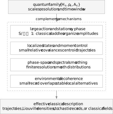
A classical-limit claim begins with a parameterized quantum family and ends with a specified effective description. Large action, localization, phase-space smoothing, and environmental decoherence are complementary rather than interchangeable.

Planck’s Constant as an Action Scale

The slogan $\hbar\to0$ is shorthand. Planck’s constant has units of action, so its bare numerical value cannot be “small” without comparison to another action.

Choose characteristic length and momentum scales $L$ and $P$, and define dimensionless variables by

$$x = L\widetilde x, \qquad p = P\widetilde p.$$

Their commutator is

$$\left[ \widetilde x, \widetilde p \right] = i\varepsilon, \qquad \varepsilon = \frac{\hbar}{LP}.$$

The combination $S_0=LP$ is a characteristic action. The semiclassical regime is

$$\varepsilon = \frac{\hbar}{S_0} \ll 1.$$

For translational motion, the same comparison can be written using the de Broglie wavelength:

$$\frac{\lambda_{\mathrm{dB}}}{L} = \frac{2\pi\hbar}{PL} = 2\pi\varepsilon.$$

Small $\varepsilon$ means that phases can vary many times across a resolved classical scale. It does not mean that commutators have been set to zero inside the original theory. Instead, one studies a family in which quantum corrections to selected dimensionless predictions become small.

Different experimental scalings can produce the same small parameter. One may increase mass, momentum, orbit size, occupation number, or action while holding suitable classical data fixed. Those are physically distinct families, and subleading corrections need not agree.

Large Quantum Numbers

Large quantum number is useful when it corresponds to large classical action. For a bound one-dimensional orbit, semiclassical quantization has the schematic form

$$J(E_n) \approx \left( n+\alpha \right)h,$$

where $J=\oint p\,dq$ is an action variable and $\alpha$ encodes turning-point or boundary information. Increasing $n$ then increases $J/\hbar$.

Relative spectral spacing

For the infinite square well,

$$E_n = \frac{n^2\pi^2\hbar^2}{2mL^2},$$

and

$$\frac{ E_{n+1}-E_n }{ E_n } = \frac{2n+1}{n^2} \longrightarrow 0.$$

The spectrum remains exactly discrete. It only becomes dense relative to the energy scale; the absolute square-well spacing actually grows with $n$. If an apparatus has fractional resolution $r$, its local bin width is of order $rE_n$. Adjacent levels are unresolved when

$$\frac{ E_{n+1}-E_n }{ E_n } \ll r,$$

but a finer apparatus may recover the discreteness.

Weak convergence rather than pointwise convergence

High-energy eigenstate densities often oscillate more rapidly rather than converging pointwise. For the $n$th harmonic-oscillator level, define its classical turning-point amplitude by

$$a_n = \sqrt{ \frac{2E_n}{m\omega^2} }.$$

In the scaled coordinate $y=x/a_n$, the classical time-spent density is

$$P_{\mathrm{cl}}(y) = \frac{1}{ \pi\sqrt{1-y^2} }, \qquad \lvert y\rvert<1.$$

A high-$n$ quantum density has many nodes and fringes. Its comparison with $P_{\mathrm{cl}}$ is naturally made after smoothing or against a slowly varying test function $g(y)$:

$$P_n(y) = a_n \lvert\psi_n(a_ny)\rvert^2.$$

Then weak convergence means

$$\begin{gathered} \int_{\mathbb R} g(y)P_n(y)\,dy\\ \longrightarrow\\ \int_{-1}^{1} g(y)P_{\mathrm{cl}}(y)\,dy. \end{gathered}$$

This is a weak, observable-dependent statement. A large-$n$ energy eigenstate does not become a particle following one orbit with a definite phase.

The canonical historical discussion is in Correspondence Principle. The detailed quantization rules live in Bohr–Sommerfeld Quantization.

Narrow Wave Packets

A localized packet supplies approximate phase-space initial data. Let

$$\overline x = \langle x\rangle, \qquad \overline p = \langle p\rangle.$$

For

$$H = \frac{p^2}{2m} + V(x),$$

Ehrenfest’s equations give

$$\frac{d\overline x}{dt} = \frac{\overline p}{m}, \qquad \frac{d\overline p}{dt} = -\langle V'(x)\rangle.$$

Newton’s equation for the centroid requires

$$\langle V'(x)\rangle \approx V'(\overline x).$$

Expanding around $\overline x$ makes the approximation quantitative. With $\delta x=x-\overline x$ and $\sigma_x^2=\langle(\delta x)^2\rangle$,

$$\begin{aligned} \langle V'(x)\rangle &= V'(\overline x) + \frac12 V'''(\overline x) \sigma_x^2\\ &\quad+ \frac16 V^{(4)}(\overline x) \langle(\delta x)^3\rangle + \cdots. \end{aligned}$$

The force correction is controlled by packet moments and derivatives of the potential. It vanishes exactly for potentials at most quadratic, but not for a generic anharmonic potential.

Spreading sets a time window

For a minimum-uncertainty free Gaussian with initial position width $\sigma_0$ and no initial position-momentum covariance,

$$\sigma_x(t)^2 = \sigma_0^2 + \left( \frac{\hbar t}{2m\sigma_0} \right)^2.$$

The dispersion time

$$t_{\mathrm{disp}} = \frac{2m\sigma_0^2}{\hbar}$$

marks when spreading becomes comparable to the initial width. Increasing the mass or initial width can lengthen this interval, but localization and small momentum uncertainty cannot both be made arbitrarily sharp because

$$\sigma_x\sigma_p \geq \frac{\hbar}{2}.$$

In nonlinear dynamics, a packet can shear, develop fine phase-space structure, or split into separated branches before simple dispersion is the dominant concern. The centroid can then cease to summarize the state even while Ehrenfest’s equations remain exact.

Ehrenfest Theorem Overview owns the theorem and its basic derivation. Gaussian Wave Packets owns the exact free-packet dynamics.

Stationary Phase

Large action explains why classical stationary paths organize many quantum amplitudes. Consider

$$I(\hbar) = \int a(q) \exp\left[ \frac{iS(q)}{\hbar} \right]dq.$$

Away from points satisfying $S'(q)=0$, nearby contributions acquire rapidly changing phases and largely cancel. Near a nondegenerate stationary point $q_k$, with $S''(q_k)\neq0$, the leading contribution is

$$\begin{aligned} I_k(\hbar) &\sim a(q_k) \sqrt{ \frac{2\pi\hbar}{ \lvert S''(q_k)\rvert } }\\ &\quad\times \exp\left[ \frac{iS(q_k)}{\hbar} \right]\\ &\quad\times \exp\left[ \frac{i\pi}{4} \operatorname{sgn}S''(q_k) \right]. \end{aligned}$$

The width of the contributing neighborhood scales as

$$\Delta q_k \sim \sqrt{ \frac{\hbar}{ \lvert S''(q_k)\rvert } }.$$

For a path integral, the analogous stationary condition is

$$\delta S[q] = 0,$$

which is the Euler–Lagrange condition for a classical path. This is why a semiclassical propagator is assembled from classical trajectories and their stability data.

Stationary phase does not usually leave one path:

• several classical paths can connect the same endpoints;
• their phases can interfere;
• stationary points can merge at caustics;
• tunneling may require complex paths or other asymptotic methods;
• nonstationary endpoint contributions can matter.

The canonical calculation is Stationary Phase. Semiclassical Propagator develops the path-based approximation.

Phase-Space Evolution

The Wigner function provides a direct comparison with classical Liouville dynamics. For

$$H(x,p) = \frac{p^2}{2m} + V(x),$$

its evolution can be expanded as

$$\begin{aligned} \frac{\partial W}{\partial t} &= -\frac{p}{m} \frac{\partial W}{\partial x} + V'(x) \frac{\partial W}{\partial p}\\ &\quad- \frac{\hbar^2}{24} V'''(x) \frac{\partial^3 W}{\partial p^3} + O(\hbar^4). \end{aligned}$$

The first row is the classical Liouville equation. The remaining Moyal terms are quantum corrections. For a quadratic Hamiltonian, derivatives beyond second order vanish, so Wigner evolution follows the classical linear phase-space flow exactly.

That exact dynamical statement has two important qualifications:

1. A Wigner function need not be a nonnegative classical probability density.
2. Even when $\hbar$ is small, rapid derivatives of $W$ can compensate the explicit powers of $\hbar$.

Fine interference fringes are therefore a warning against judging the classical limit by coefficients alone. One must control both the equation and the family of states to which it is applied.

Classical Limit of the Moyal Bracket owns the phase-space expansion. Wigner Function develops its probabilistic strengths and limitations.

Decoherence

Semiclassical dynamics can explain trajectories and phase-space flow, but a classical world also contains records that are stable and do not visibly interfere. Environmental decoherence addresses this second task.

Suppose two orthonormal system alternatives become correlated with environmental records:

$$\begin{aligned} &\left( c_1\lvert s_1\rangle + c_2\lvert s_2\rangle \right) \lvert E_0\rangle\\ &\qquad\longrightarrow c_1\lvert s_1\rangle\lvert E_1\rangle + c_2\lvert s_2\rangle\lvert E_2\rangle. \end{aligned}$$

Define the decoherence factor

$$\gamma = \langle E_2\mid E_1\rangle.$$

After tracing out the environment, the system state is

$$\rho_S = \begin{pmatrix} \lvert c_1\rvert^2 & c_1c_2^*\gamma\\ c_1^*c_2\gamma^* & \lvert c_2\rvert^2 \end{pmatrix}.$$

When $\lvert\gamma\rvert\ll1$, local interference between the alternatives is suppressed. The interaction also tends to select robust pointer states: states whose correlations survive environmental monitoring better than generic superpositions.

This explains why certain bases support stable records and why recovering macroscopic interference becomes extraordinarily difficult. It does not justify replacing the global entangled state by one realized branch without additional measurement or interpretive input. Nor is decoherence identical to energy dissipation: phase coherence can be lost on a timescale very different from energy relaxation.

Decoherence Preview gives the Core bridge. Environment-Induced Decoherence is the canonical open-systems treatment.

Coarse Graining

Classical predictions are usually made at finite resolution. A detector reports a region $\Delta$, not an infinitely sharp phase-space point. In quantum language, that report is represented by an effect $E_\Delta$ with

$$\Pr(\Delta) = \operatorname{Tr} \left( \rho E_\Delta \right).$$

Coarse graining can suppress sensitivity to structures much finer than the measurement scale. A smoothed phase-space function can be written schematically as

$$\overline W_\sigma(z) = \int G_\sigma(z-z') W(z')\,dz',$$

where $G_\sigma$ is a resolution kernel. Oscillations on scales much smaller than $\sigma$ average out.

This mechanism explains why a sequence may converge only through finite resolution or weak observables. In the square well, for example,

$$\sin^2\left( \frac{n\pi x}{L} \right) = \frac12 - \frac12 \cos\left( \frac{2n\pi x}{L} \right).$$

The cosine term does not approach zero pointwise as $n\to\infty$, but its average against a smooth, fixed-resolution response tends to zero.

Coarse graining and decoherence must not be conflated:

• coarse graining restricts which distinctions are observed or retained;
• decoherence is a dynamical transfer of phase information into correlations with an environment.

Either can make interference locally inaccessible. In the distinction used here, only the decoherence step invokes an actual system–environment interaction that changes the subsystem’s reduced state.

Worked Synthesis: A Harmonic-Oscillator Coherent State

A coherent state shows several mechanisms working together without being identical. Let

$$a\lvert\alpha\rangle = \alpha\lvert\alpha\rangle.$$

Its mean occupation and fluctuation are

$$\langle N\rangle = \lvert\alpha\rvert^2, \qquad \Delta N = \lvert\alpha\rvert.$$

Hence

$$\frac{\Delta N}{\langle N\rangle} = \frac{1}{\lvert\alpha\rvert},$$

which is small for $\lvert\alpha\rvert\gg1$. The position centroid follows the exact classical orbit

$$\overline x(t) = \sqrt{ \frac{2\hbar}{m\omega} } \lvert\alpha\rvert \cos\left( \omega t-\arg\alpha \right),$$

while the width remains

$$\Delta x = \sqrt{ \frac{\hbar}{2m\omega} }.$$

At the turning point, the relative width is

$$\frac{\Delta x}{x_{\mathrm{amp}}} = \frac{1}{2\lvert\alpha\rvert}.$$

This state therefore has:

• large action when $\lvert\alpha\rvert^2\gg1$;
• a narrow relative phase-space distribution;
• an exactly classical centroid because the Hamiltonian is quadratic;
• small relative number fluctuations.

Yet the state remains a pure quantum state and can interfere with another coherent state. No environment was needed to obtain its classical centroid. Decoherence becomes relevant when asking why separated alternatives or apparatus records fail to interfere locally.

Coherent States owns their construction and exact dynamics.

Timescales and Breakdown

A useful classical approximation carries a clock. Relevant times may include:

• $t_{\mathrm{dyn}}$, the classical dynamical period;
• $t_{\mathrm{disp}}$, the wave-packet spreading time;
• $t_{\mathrm{nl}}$, the time for nonlinear distortion or branching;
• $t_{\mathrm{dec}}$, the decoherence time in a selected basis;
• $t_{\mathrm{rel}}$, the energy-relaxation time;
• $t_{\mathrm{rec}}$, a recurrence or revival time;
• $t_{\mathrm{obs}}$, the experimental observation window.

There is no universal ordering. A classical record regime often relies on decoherence being fast compared with observation,

$$t_{\mathrm{dec}} \ll t_{\mathrm{obs}},$$

while trajectory accuracy requires the observation window to remain shorter than the relevant packet or semiclassical breakdown time.

In classically chaotic systems, nearby trajectories separate exponentially. A representative semiclassical estimate for the Ehrenfest time is

$$t_{\mathrm E} \sim \frac{1}{\lambda} \log\left( \frac{S_0}{\hbar} \right),$$

where $\lambda$ is a positive Lyapunov exponent. The precise coefficient and applicability depend on the system and observable, but the logarithm conveys an important lesson: making $S_0/\hbar$ enormous does not necessarily make a single-packet trajectory accurate forever.

Long-time and small-parameter limits may therefore fail to commute:

$$\lim_{\varepsilon\to0} \lim_{t\to\infty} \neq \lim_{t\to\infty} \lim_{\varepsilon\to0}.$$

Claims about “the” classical limit should never silently exchange these orders.

What Kind of Classical Theory Emerges?

The output need not be Newton’s equation for one point particle.

Quantum regime	Natural classical description
Narrow packet under a smooth near-quadratic potential	Approximate Hamiltonian trajectory
Incoherent or uncertain preparation	Liouville ensemble on phase space
Open system with weak noise	Stochastic differential or kinetic equation
Highly occupied bosonic mode	Classical complex amplitude or field
Short wavelength wave propagation	Ray or eikonal description
Decohered measuring apparatus	Stable alternatives and classical records

Classical statistical mechanics is already a classical theory. Obtaining a probability distribution rather than a single trajectory is not a failure of the limit. The target must match the preparation and the observables actually resolved.

A Practical Classical-Limit Audit

Before accepting a classical approximation, ask:

1. What quantum family is being scaled?
2. Which dimensionless parameter tends to zero or infinity?
3. Which classical quantities remain fixed?
4. Is the target a trajectory, ensemble, field, stochastic process, or record?
5. Which observables and detector resolutions define agreement?
6. Does the state remain localized in the relevant variables?
7. Are Moyal, WKB, or stationary-phase corrections controlled?
8. Is environmental decoherence being assumed, modeled, or ignored?
9. What error estimate and time window support the claim?
10. Could a finer measurement reveal the discarded quantum structure?

This audit turns “classical behavior” from a slogan into a testable approximation statement.

Why No Single Slogan Is Enough

Several common implications are false:

$$S/\hbar\gg1 \;\not\Rightarrow\; \text{one localized trajectory},$$ $$n\gg1 \;\not\Rightarrow\; \text{pointwise classical density},$$

and

$$\begin{gathered} \text{decoherence}\\ \not\Rightarrow\\ \text{unique realized outcome}. \end{gathered}$$

Conversely, a system need not be large in geometric size to have a useful classical description. Highly occupied field modes, collective spins, and small mechanical resonators can display classical behavior for selected observables, while macroscopic systems can retain detectable quantum coherence under sufficient isolation and control.

Common Misstatements About the Classical Limit provides the full myth-correction guide. Quantization vs Classical Limit explains why constructing a quantum model from classical data is the opposite direction and is not a literal inverse operation.

Connections

• Semiclassical Limit Overview introduces WKB and path-integral stationary phase.
• Semiclassical Limits and Correspondence gives the method-level rules for scaled families, errors, and observables.
• Phase Space defines the classical state space used in trajectory and ensemble limits.
• Why Phase Space? connects operator dynamics with quasiprobability evolution.
• Environment-Induced Decoherence owns dynamical suppression of local coherence and pointer-state selection.

Common Mistakes

• Treating $\hbar\to0$ as dimensional arithmetic rather than a scaled family.
• Assuming large quantum number makes every eigenstate a trajectory.
• Comparing oscillatory densities pointwise when only weak convergence is justified.
• Using Ehrenfest’s theorem without tracking packet moments and spreading.
• Keeping only the first Moyal term while the Wigner function develops fine derivatives.
• Reading stationary phase as proof that exactly one classical path occurred.
• Treating detector coarse graining and environmental decoherence as the same process.
• Treating a diagonal reduced density matrix as proof of one realized outcome.
• Omitting the observation time from an approximation claim.
• Assuming the classical limit must be deterministic rather than statistical.

References

• N. Bohr, “On the Quantum Theory of Line-Spectra,” Det Kongelige Danske Videnskabernes Selskabs Skrifter 8, 4, 1–118 (1918).
• L. E. Ballentine, Quantum Mechanics: A Modern Development, 2nd ed., World Scientific (2014).
• L. D. Landau and E. M. Lifshitz, Quantum Mechanics: Non-Relativistic Theory, 3rd ed., Pergamon (1977).
• M. V. Berry and K. E. Mount, “Semiclassical approximations in wave mechanics,” Reports on Progress in Physics 35, 315–397 (1972), doi:10.1088/0034-4885/35/1/306.
• R. G. Littlejohn, “The semiclassical evolution of wave packets,” Physics Reports 138, 193–291 (1986), doi:10.1016/0370-1573(86)90103-1.
• M. Brack and R. K. Bhaduri, Semiclassical Physics, 2nd ed., Westview Press (2003).
• W. H. Zurek, “Decoherence, einselection, and the quantum origins of the classical,” Reviews of Modern Physics 75, 715–775 (2003), doi:10.1103/RevModPhys.75.715.
• M. Schlosshauer, “Decoherence, the measurement problem, and interpretations of quantum mechanics,” Reviews of Modern Physics 76, 1267–1305 (2005), doi:10.1103/RevModPhys.76.1267.
• M. Schlosshauer, Decoherence and the Quantum-to-Classical Transition, 2nd ed., Springer (2019).

Exercises

1. Let $x=L\widetilde x$ and $p=P\widetilde p$. Derive the commutator of the dimensionless variables and identify the parameter that controls the semiclassical regime.

Solution

Using $[x,p]=i\hbar$,

$$\begin{aligned} \left[ \widetilde x, \widetilde p \right] &= \left[ \frac{x}{L}, \frac{p}{P} \right]\\ &= \frac{i\hbar}{LP}. \end{aligned}$$

Therefore

$$\left[ \widetilde x, \widetilde p \right] = i\varepsilon, \qquad \varepsilon = \frac{\hbar}{LP}.$$

The quantity $LP$ is a characteristic action. The semiclassical regime for these scales is $\varepsilon\ll1$, not a unit-dependent statement that $\hbar$ itself is numerically small.

2. An infinite-square-well apparatus has fractional energy resolution $r$, so its bin width near $E_n$ is approximately $rE_n$. Find the condition under which adjacent levels near $n$ are unresolved, and explain why this does not make the exact spectrum continuous.

Solution

For

$$E_n = \frac{n^2\pi^2\hbar^2}{2mL^2},$$

the spacing is

$$E_{n+1}-E_n = \frac{(2n+1)\pi^2\hbar^2}{2mL^2}.$$

Adjacent levels are experimentally unresolved when

$$\frac{ E_{n+1}-E_n }{ E_n } = \frac{2n+1}{n^2} \ll r.$$

The measurement then groups several exact eigenvalues into one reported energy bin. The Hamiltonian’s spectrum remains discrete; only the finite-resolution description is effectively continuous.

3. Expand $\langle V'(x)\rangle$ around $\overline x=\langle x\rangle$ through second central order. State a quantitative condition for Newtonian centroid motion.

Solution

Write $x=\overline x+\delta x$, where $\langle\delta x\rangle=0$. Taylor expansion gives

$$\begin{aligned} V'(x) &= V'(\overline x) + V''(\overline x)\delta x\\ &\quad+ \frac12 V'''(\overline x)(\delta x)^2 + \cdots. \end{aligned}$$

Taking the expectation value removes the linear central moment:

$$\langle V'(x)\rangle = V'(\overline x) + \frac12 V'''(\overline x)\sigma_x^2 + \cdots.$$

When a nonzero local force scale is appropriate, one useful condition is

$$\frac{ \lvert V'''(\overline x)\rvert \sigma_x^2 }{ 2\lvert V'(\overline x)\rvert } \ll 1,$$

together with control of higher central moments. Near a point where $V'(\overline x)=0$, the correction should instead be compared with a problem-specific force or acceleration scale.

4. A minimum-uncertainty free Gaussian begins with width $\sigma_0$. At what time has its variance doubled? What does the mass dependence imply?

Solution

The variance is

$$\sigma_x(t)^2 = \sigma_0^2 + \left( \frac{\hbar t}{2m\sigma_0} \right)^2.$$

Setting $\sigma_x(t)^2=2\sigma_0^2$ gives

$$t = \frac{2m\sigma_0^2}{\hbar} = t_{\mathrm{disp}}.$$

At fixed initial width, increasing the mass lengthens the spreading time. This helps a massive packet remain localized over a fixed observation window, but it does not remove uncertainty or guarantee classical behavior in an arbitrary potential.

5. Near a stationary point, approximate

$$S(q) \approx S(q_0) + \frac12 S''(q_0)(q-q_0)^2.$$

Use phase variation to estimate the width of the region that contributes coherently.

Solution

The phase relative to $q_0$ is approximately

$$\Delta\varphi \approx \frac{ S''(q_0)(q-q_0)^2 }{ 2\hbar }.$$

Coherent contributions come from the region where this phase is of order one or smaller. Therefore

$$\lvert q-q_0\rvert \sim \sqrt{ \frac{\hbar}{ \lvert S''(q_0)\rvert } },$$

up to a constant of order one. This shrinking neighborhood underlies the stationary-phase approximation.

6. Why does the Moyal evolution equation reduce exactly to the classical Liouville equation for a quadratic potential? Does this prove that every state is a classical probability distribution?

Solution

All Moyal corrections beyond the Poisson-bracket term contain third or higher derivatives of $V$. For a quadratic potential,

$$V'''(x) = V^{(4)}(x) = \cdots = 0,$$

so those dynamical corrections vanish exactly.

This does not make every Wigner function a classical probability density. Nonclassical initial states can have negative or oscillatory Wigner functions. Quadratic evolution transports that structure by the classical linear phase-space flow without converting it into a positive probability density.

7. For the two-branch decoherence model, show that the magnitude of each off-diagonal element of $\rho_S$ is multiplied by $\lvert\gamma\rvert=\lvert\langle E_2\mid E_1\rangle\rvert$. What happens when the environmental states are equal or orthogonal?

Solution

Tracing the joint state over the environment gives off-diagonal elements

$$\rho_{12} = c_1c_2^* \langle E_2\mid E_1\rangle = c_1c_2^*\gamma$$

and

$$\rho_{21} = c_1^*c_2\gamma^*.$$

Their magnitudes are reduced by $\lvert\gamma\rvert$. If $\lvert E_1\rangle=\lvert E_2\rangle$, then $\gamma=1$ and the environment stores no which-branch information. If the records are orthogonal, then $\gamma=0$ and local off-diagonal terms vanish exactly in this basis.

8. Diagnose the mechanisms needed in each case: a high-$n$ box energy measurement with poor resolution; a coherent oscillator whose centroid is tracked for one period; two spatially separated apparatus pointer states; and a path-integral propagator with several classical paths.

Solution

The poorly resolved box spectrum uses large relative quantum number together with energy coarse graining. It does not require a localized trajectory.

The coherent oscillator uses large action, small relative fluctuations, and exact quadratic centroid dynamics. Decoherence is unnecessary for predicting the isolated centroid over one period.

Separated apparatus pointer states require open-system dynamics and decoherence to explain suppression of locally observable interference and stability of the record basis. That mechanism alone does not select one actual outcome.

The propagator uses stationary phase. Every relevant stationary classical path contributes with an amplitude, stability factor, and phase; the paths must be summed rather than replaced by a unique classical history.