Breit–Wigner Form

The Breit–Wigner form is the universal leading description of an isolated, narrow resonance. In its simplest elastic partial-wave form,

$$S_\ell(E) = e^{2i\delta_{\ell,\mathrm{bg}}(E)} \frac{ E-E_R-i\Gamma/2 }{ E-E_R+i\Gamma/2 }.$$

The factor has a pole at $E_R-i\Gamma/2$, advances the resonant phase by $\pi$, and produces a Lorentzian cross-section profile when the background is negligible. The two parameters are an energy $E_R$ and a full width at half maximum $\Gamma$.

The formula is powerful because it ties together four descriptions of the same local structure:

• a pole of the analytically continued amplitude;
• rapid phase motion on the real energy axis;
• a peak or peak–dip structure in an observable;
• a lifetime scale $\hbar/\Gamma$.

It is not a universal fit function for every bump. Thresholds, energy-dependent phase space, nonresonant backgrounds, overlapping poles, and coupled channels can all deform the elementary profile.

Resonances owns the physical classification of quasibound and resonant states. Bound States and Scattering Poles owns their placement on analytically continued energy and momentum sheets. This page is the canonical home for the Breit–Wigner parameterization itself, including its derivation, observables, diagnostics, and domain of validity.

Scope and Assumptions

Begin with distinguishable spinless particles in one elastic partial wave $\ell$. Assume:

1. one resonance pole is much closer to the physical energy region than other poles;
2. no threshold or branch point lies within a few widths of the resonance;
3. nonresonant factors vary slowly across an interval of order $\Gamma$;
4. the resonance is narrow enough that $k(E)$ and other kinematic prefactors can be evaluated at $E_R$ when deriving the elementary line shape.

The useful control ratio is schematically

$$\frac{\Gamma}{\Delta}\ll1,$$

where $\Delta$ is the energy distance to the nearest omitted singularity or comparably rapid dynamical structure. A smooth background need not be small, but its variation across the resonance should be small:

$$\Gamma \left| \frac{d\delta_{\ell,\mathrm{bg}}}{dE} \right| \ll1.$$

These conditions are more informative than saying only that the peak “looks narrow.”

Unitary Pole Factor

Write

$$x=E-E_R, \qquad \gamma=\frac{\Gamma}{2}.$$

The resonant factor is

$$S_{\mathrm{res}}(E) = \frac{x-i\gamma}{x+i\gamma}.$$

For real $E$,

$$\left| S_{\mathrm{res}}(E) \right|=1,$$

so this factor is exactly elastic-unitary. Its analytic continuation has

$$\begin{aligned} \text{pole:}\quad E_p &= E_R-i\frac{\Gamma}{2}, \\ \text{zero:}\quad E_z &= E_R+i\frac{\Gamma}{2}. \end{aligned}$$

The lower-half-plane pole gives decay rather than exponential growth. In a continuum problem it lies on the sheet reached by analytically continuing through the appropriate threshold cut. The conjugate zero is required by the real-axis unitarity of this one-channel factor.

The full elastic element may contain a smooth phase:

$$S_\ell(E) = e^{2i\delta_{\ell,\mathrm{bg}}(E)} S_{\mathrm{res}}(E).$$

Multiplication is essential. Simply adding a pole term to an arbitrary background does not automatically preserve $\lvert S_\ell\rvert=1$.

Phase-Shift Form

Define the resonant phase through

$$S_{\mathrm{res}}(E) = e^{2i\delta_{\mathrm{res}}(E)}.$$

Comparison with the pole factor gives

$$\cot\delta_{\mathrm{res}}(E) = \frac{E_R-E}{\Gamma/2}.$$

A continuous branch can be chosen so that

$$\delta_{\mathrm{res}}(E) = \frac{\pi}{2} + \arctan \left( \frac{2(E-E_R)}{\Gamma} \right).$$

It then obeys

$$\begin{aligned} \delta_{\mathrm{res}} &\longrightarrow 0 && (E\ll E_R), \\ \delta_{\mathrm{res}}(E_R) &= \frac{\pi}{2}, \\ \delta_{\mathrm{res}} &\longrightarrow \pi && (E\gg E_R). \end{aligned}$$

The phase therefore advances by $\pi$ across an isolated resonance. A displayed principal-value arctangent may jump by $\pi$ even though the physical phase is continuous; phase unwrapping is part of the analysis, not an optional plotting choice.

The complete phase shift is

$$\delta_\ell(E) = \delta_{\ell,\mathrm{bg}}(E) + \delta_{\mathrm{res}}(E).$$

A resonance is diagnosed more reliably by this rapid phase motion or by a nearby pole than by a peak alone.

Amplitude and Elastic Line Shape

Use the dimensionless partial-wave amplitude

$$a_\ell(E) = \frac{S_\ell(E)-1}{2i}.$$

With no background phase,

$$\begin{aligned} a_\ell^{\mathrm{res}}(E) &= \frac{1}{2i} \left( \frac{x-i\gamma}{x+i\gamma} -1 \right) \\ &= -\frac{\gamma}{x+i\gamma}. \end{aligned}$$

At $E=E_R$,

$$a_\ell^{\mathrm{res}}(E_R)=i,$$

which lies at the top of the elastic unitarity circle. Its magnitude is

$$\left| a_\ell^{\mathrm{res}}(E) \right|^2 = \frac{\Gamma^2/4}{ (E-E_R)^2+\Gamma^2/4 }.$$

For distinguishable spinless particles, the elastic contribution of this partial wave is therefore

$$\sigma_\ell^{\mathrm{el}}(E) = \frac{4\pi}{k^2} (2\ell+1) \frac{\Gamma^2/4}{ (E-E_R)^2+\Gamma^2/4 }.$$

If $k$ is nearly constant across the resonance, the peak reaches

$$\sigma_\ell^{\max} = \frac{4\pi}{k_R^2} (2\ell+1), \qquad k_R=k(E_R).$$

This is the one-channel elastic unitarity limit. Partial-Wave Cross Sections derives the general channel sums and their bounds.

Full Width at Half Maximum

Introduce the dimensionless detuning

$$\varepsilon = \frac{2(E-E_R)}{\Gamma}.$$

The normalized line shape is

$$L(\varepsilon) = \frac{ \sigma_\ell^{\mathrm{el}}(E) }{ \sigma_\ell^{\max} } = \frac{1}{1+\varepsilon^2}.$$

Half maximum occurs at

$$\varepsilon=\pm1,$$

or

$$E=E_R\pm\frac{\Gamma}{2}.$$

The distance between these two energies is $\Gamma$, which is why $\Gamma$ is the full width at half maximum. The half width at half maximum is $\Gamma/2$.

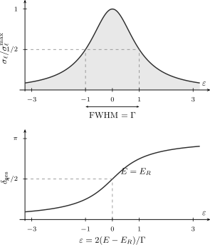
For an isolated elastic resonance with negligible background, the same detuning controls the Lorentzian cross section and the continuous $\pi$ phase advance. The half-maximum points lie at $E_R\pm\Gamma/2$.

The elementary profile is symmetric about $E_R$. An observed asymmetric profile is not evidence against a resonance; it is evidence that amplitudes other than the isolated pole are contributing coherently or that nearby kinematics vary appreciably.

Pole Width and Lifetime

The pole energy

$$E_p = E_R-i\frac{\Gamma}{2}$$

produces the time factor

$$\begin{aligned} \exp \left( -\frac{iE_p t}{\hbar} \right) &= \exp \left( -\frac{iE_R t}{\hbar} \right) \\ &\quad\times \exp \left( -\frac{\Gamma t}{2\hbar} \right). \end{aligned}$$

The corresponding probability decays as

$$P(t)\propto e^{-\Gamma t/\hbar},$$

so the exponential lifetime is

$$\tau=\frac{\hbar}{\Gamma}.$$

This relation concerns the pole decay law. It should not be identified term by term with every collision-time definition.

For example, the one-channel Wigner–Smith delay is

$$\tau_{\mathrm W}(E) = 2\hbar \frac{d\delta_\ell}{dE}.$$

With a constant width and negligible background,

$$\frac{d\delta_{\mathrm{res}}}{dE} = \frac{\Gamma/2}{ (E-E_R)^2+\Gamma^2/4 },$$

and hence

$$\tau_{\mathrm W}(E_R) = \frac{4\hbar}{\Gamma}.$$

The factor of four relative to $\hbar/\Gamma$ is not a contradiction. The Wigner–Smith quantity compares scattering phases and wave-packet arrival times, whereas $\hbar/\Gamma$ is the exponential survival lifetime of the pole state.

Background Interference

Let the background phase be approximately constant over the resonance. The elastic partial cross section remains

$$\sigma_\ell^{\mathrm{el}}(E) = \frac{4\pi}{k^2} (2\ell+1) \sin^2 \left( \delta_{\ell,\mathrm{bg}} + \delta_{\mathrm{res}} \right).$$

For the detuning $\varepsilon$ defined above,

$$\begin{aligned} \sin\delta_{\mathrm{res}} &= \frac{1}{\sqrt{1+\varepsilon^2}}, \\ \cos\delta_{\mathrm{res}} &= -\frac{\varepsilon}{ \sqrt{1+\varepsilon^2} }. \end{aligned}$$

For compactness in the next formulas, write

$$\delta_{\mathrm{bg}} \equiv \delta_{\ell,\mathrm{bg}}.$$

Then

$$\begin{aligned} & \sin^2 \left( \delta_{\mathrm{bg}} + \delta_{\mathrm{res}} \right) \\ &\qquad= \frac{ \left( \cos\delta_{\mathrm{bg}} - \varepsilon\sin\delta_{\mathrm{bg}} \right)^2 }{ 1+\varepsilon^2 }. \end{aligned}$$

Three consequences follow immediately:

• at $E=E_R$, the cross-section factor is $\cos^2\delta_{\ell,\mathrm{bg}}$, not necessarily one;
• elastic saturation occurs at

$$E_{\max} = E_R - \frac{\Gamma}{2} \tan\delta_{\ell,\mathrm{bg}};$$

• a zero can occur at

$$E_{\mathrm{zero}} = E_R + \frac{\Gamma}{2} \cot\delta_{\ell,\mathrm{bg}}.$$

The same pole can therefore produce a displaced peak, an asymmetric peak–dip profile, or primarily a dip. This is amplitude interference. The Fano profile is a standard broader framework for such asymmetric resonance shapes.

Partial Widths and Several Channels

Suppose an isolated state couples to open channels $a,b,\ldots$. Assign a partial width $\Gamma_c$ to each open decay channel and define

$$\Gamma = \sum_c\Gamma_c.$$

Ignoring smooth channel phases for the moment, a unitary resonant channel matrix can be written locally as

$$S_{ba}(E) = \delta_{ba} - \frac{ i\sqrt{\Gamma_b\Gamma_a} }{ E-E_R+i\Gamma/2 }.$$

For one channel, $\Gamma_a=\Gamma$, and this reduces to the elastic pole factor. The factorized numerator expresses the fact that the state must be formed from channel $a$ and then decay into channel $b$.

For spinless scattering in a definite partial wave, the resonant transition cross section has the form

$$\begin{aligned} \sigma_{a\to b}^{(\ell)}(E) &= \frac{\pi}{k_a^2} (2\ell+1) \\ &\quad\times \frac{ \Gamma_a\Gamma_b }{ (E-E_R)^2+\Gamma^2/4 }. \end{aligned}$$

Introduce branching fractions

$$B_c=\frac{\Gamma_c}{\Gamma}.$$

Then

$$\begin{aligned} \sigma_{a\to b}^{(\ell)}(E) &= \frac{4\pi}{k_a^2} (2\ell+1) \\ &\quad\times \frac{ \Gamma^2/4 }{ (E-E_R)^2+\Gamma^2/4 } B_aB_b. \end{aligned}$$

The resonance may be narrow yet weak in a chosen reaction because either its entrance or exit branching fraction is small.

For a resonance of total angular momentum $J$ formed by incident spins $s_1$ and $s_2$, the commonly used unpolarized formation formula is

$$\begin{aligned} \sigma_{a\to b}(E) &= \frac{2J+1}{ (2s_1+1)(2s_2+1) } \frac{4\pi}{k_a^2} \\ &\quad\times \frac{ \Gamma^2/4 }{ (E-E_R)^2+\Gamma^2/4 } B_aB_b. \end{aligned}$$

Additional symmetry, polarization, identical-particle, and channel-normalization factors must be restored for the process at hand. The scalar formula is a convention dictionary, not a substitute for deriving the measured observable.

Thresholds and Energy-Dependent Widths

A constant width is inappropriate when an open-channel momentum changes appreciably across the resonance. For a short-range two-body channel $c$ with orbital angular momentum $\ell_c$, threshold behavior gives schematically

$$\Gamma_c(E) \propto k_c(E)^{2\ell_c+1}$$

above threshold. The total width becomes

$$\Gamma(E) = \sum_c\Gamma_c(E).$$

A more realistic local denominator then has the structure

$$D(E) = E-E_0-\Delta(E) + \frac{i}{2}\Gamma(E),$$

where $\Delta(E)$ is an energy shift associated with the real part of the self-energy. Analyticity links $\Delta(E)$ and $\Gamma(E)$; changing only the imaginary part may be an expedient model but is not a complete analytic construction.

Near an $s$-wave threshold, $k_c(E)$ has square-root behavior. The resulting cusp or rapid width variation can invalidate a symmetric Lorentzian even when a pole is present. A nearby closed or newly opened channel may require a coupled-channel parameterization rather than a constant-width Breit–Wigner form.

The practical criterion is not simply $\Gamma/E_R\ll1$. One also needs

$$\Gamma \ll \Delta_{\mathrm{threshold}},$$

unless the threshold dependence is included explicitly and analytically.

Relativistic Translation

In particle physics, an invariant-mass amplitude is often written schematically as

$$\operatorname{BW}(s) = \frac{1}{ m_{\mathrm{BW}}^2-s - i m_{\mathrm{BW}}\Gamma(s) }.$$

Here $s$ is the squared center-of-mass energy. For $\sqrt{s}=E$ close to $m_{\mathrm{BW}}$,

$$m_{\mathrm{BW}}^2-s \simeq -2m_{\mathrm{BW}} \left( E-m_{\mathrm{BW}} \right),$$

so the squared denominator reduces locally to the nonrelativistic Lorentzian after removal of a smooth overall factor.

Several distinctions matter:

• $m_{\mathrm{BW}}$ and $\Gamma_{\mathrm{BW}}$ are parameters of a chosen real-axis parameterization;
• a pole is defined by a complex solution $s_p$ of the analytically continued denominator;
• pole mass and width may be introduced through

$$\sqrt{s_p} = M_p-i\frac{\Gamma_p}{2};$$

• Breit–Wigner and pole parameters agree closely only for a sufficiently narrow, isolated resonance with mild energy dependence;
• numerators contain production couplings, spin tensors, barrier factors, and channel phase space, so the observed invariant-mass distribution is not just $\lvert\operatorname{BW}(s)\rvert^2$.

Bridge to QFT Scattering places resonance poles in relativistic amplitudes. QFT Bridge: Optical Theorem and Unitarity explains the corresponding relativistic unitarity constraints.

Narrow-Width Limit

The normalized Lorentzian satisfies

$$\lim_{\Gamma\to0^+} \frac{1}{\pi} \frac{\Gamma/2}{ (E-E_R)^2+\Gamma^2/4 } = \delta(E-E_R)$$

in the distributional sense. Consequently,

$$\frac{\Gamma^2/4}{ (E-E_R)^2+\Gamma^2/4 } \longrightarrow \frac{\pi\Gamma}{2} \delta(E-E_R).$$

This replacement is valid only inside an integral whose remaining factors are smooth across the width. It turns resonant production and decay into an on-shell factorization:

$$\text{production} \times \text{branching fraction}.$$

It fails when cuts, selection thresholds, detector response, parton luminosities, or interference vary significantly over the resonant region.

Worked Checks

Isolated p-wave resonance

Take $\ell=1$, $k_R=2\,\mathrm{fm}^{-1}$, and $\Gamma=4\,\mathrm{MeV}$. The elastic peak is

$$\begin{aligned} \sigma_1^{\max} &= \frac{4\pi}{(2\,\mathrm{fm}^{-1})^2} (3) \\ &= 3\pi\,\mathrm{fm}^2 \simeq 9.42\,\mathrm{fm}^2. \end{aligned}$$

Since $1\,\mathrm{fm}^2=10\,\mathrm{mb}$, this is about $94.2\,\mathrm{mb}$. The half-maximum energies are $E_R\pm2\,\mathrm{MeV}$.

Smooth background phase

Let $\delta_{\ell,\mathrm{bg}}=\pi/6$. At the pole-energy parameter,

$$\frac{ \sigma_\ell(E_R) }{ \sigma_\ell^{\max} } = \cos^2\frac{\pi}{6} = \frac{3}{4}.$$

The elastic maximum is shifted to

$$E_{\max} = E_R - \frac{\Gamma}{2\sqrt{3}}.$$

The pole position has not moved in this constant-background model. The peak has moved because the observable depends on coherent phase addition.

Channel suppression

If $B_a=0.10$ and $B_b=0.25$, then the peak cross section for $a\to b$ is only

$$B_aB_b=0.025$$

times the spin-weighted unitarity prefactor. A prominent pole can therefore be inconspicuous in one final state and clear in another.

Diagnostic Workflow

When using a Breit–Wigner form:

1. Specify the amplitude convention. State whether the denominator is written in $E$, $k$, or $s$, and define every numerator factor.
2. Locate nearby singularities. Compare $\Gamma$ with distances to thresholds and other poles.
3. Check phase motion. A genuine isolated elastic resonance advances the phase rapidly; a peak without compatible phase behavior may be kinematic or interference driven.
4. Preserve unitarity. Use a multiplicative elastic factor or a coupled-channel construction with the correct total width.
5. Allow the width to vary when required. Restore threshold powers and phase space before fitting near an opening channel.
6. Fit amplitudes coherently. Add complex amplitudes, not separately squared resonance yields.
7. Report the parameter definition. Distinguish Breit–Wigner parameters from analytically continued pole parameters.
8. Stress-test the model. Vary the background, fit window, width prescription, and included channels.

Common Mistakes

• Calling $\Gamma/2$ the full width.
• Using a principal arctangent without unwrapping the phase through $\pi$.
• Assuming the cross-section maximum must occur at $E_R$ in the presence of background interference.
• Adding several Breit–Wigner amplitudes in one partial wave without checking unitarity.
• Holding $\Gamma$ constant across a nearby threshold.
• Treating $\hbar/\Gamma$ and the peak Wigner–Smith delay as identical times.
• Equating fitted Breit–Wigner mass and width with pole mass and width for a broad state.
• Applying the narrow-width delta function when other factors vary on the scale $\Gamma$.
• Fitting a histogram with a bare Lorentzian while ignoring resolution, acceptance, phase space, and coherent background.

Exercises

1. Verify that the elastic resonant factor

$$S_{\mathrm{res}}(E) = \frac{E-E_R-i\Gamma/2}{ E-E_R+i\Gamma/2 }$$

has unit magnitude for real $E$. Locate its pole and zero.

Solution

For real $E$, the numerator is the complex conjugate of the denominator, so

$$\left| S_{\mathrm{res}} \right|^2 = \frac{ (E-E_R)^2+\Gamma^2/4 }{ (E-E_R)^2+\Gamma^2/4 } =1.$$

The denominator vanishes at

$$E=E_R-i\frac{\Gamma}{2},$$

which is the pole. The numerator vanishes at

$$E=E_R+i\frac{\Gamma}{2},$$

which is the conjugate zero.

2. Starting from

$$L(E) = \frac{\Gamma^2/4}{ (E-E_R)^2+\Gamma^2/4 },$$

show that the full width at half maximum is $\Gamma$.

Solution

The maximum is $L(E_R)=1$. Set $L(E)=1/2$:

$$\frac{\Gamma^2/4}{ (E-E_R)^2+\Gamma^2/4 } = \frac12.$$

Cross-multiplication gives

$$(E-E_R)^2 = \frac{\Gamma^2}{4}.$$

Thus the two half-maximum points are $E_R-\Gamma/2$ and $E_R+\Gamma/2$. Their separation is $\Gamma$.

3. Assume a constant background phase $\delta_{\mathrm{bg}}$. Derive the energy at which the elastic channel saturates its unitarity bound.

Solution

Saturation requires

$$\delta_{\mathrm{bg}} + \delta_{\mathrm{res}} = \frac{\pi}{2} \pmod{\pi}.$$

For the branch through the resonance,

$$\delta_{\mathrm{res}} = \frac{\pi}{2} - \delta_{\mathrm{bg}}.$$

Using

$$\cot\delta_{\mathrm{res}} = \frac{E_R-E}{\Gamma/2}$$

and

$$\cot \left( \frac{\pi}{2} - \delta_{\mathrm{bg}} \right) = \tan\delta_{\mathrm{bg}},$$

one obtains

$$E_{\max} = E_R - \frac{\Gamma}{2} \tan\delta_{\mathrm{bg}}.$$

The observed maximum can therefore differ from the pole-energy parameter even when the background is constant.

4. A resonance has branching fractions $B_a=1/4$ into its entrance channel and $B_b=1/2$ into an observed exit channel. At $E=E_R$, what fraction of the spin-weighted unitarity prefactor appears in $\sigma_{a\to b}$?

Solution

At $E_R$, the Lorentzian factor is one. The remaining channel factor is

$$B_aB_b = \frac14\frac12 = \frac18.$$

Thus the resonant transition reaches one eighth of the relevant spin-weighted unitarity prefactor.

5. Derive the peak Wigner–Smith delay for the constant-width resonance and compare it with the exponential lifetime.

Solution

Differentiate the continuous resonant phase:

$$\frac{d\delta_{\mathrm{res}}}{dE} = \frac{\Gamma/2}{ (E-E_R)^2+\Gamma^2/4 }.$$

At $E_R$,

$$\left. \frac{d\delta_{\mathrm{res}}}{dE} \right|_{E_R} = \frac{2}{\Gamma}.$$

Therefore

$$\tau_{\mathrm W}(E_R) = 2\hbar \left. \frac{d\delta_{\mathrm{res}}}{dE} \right|_{E_R} = \frac{4\hbar}{\Gamma}.$$

The pole survival lifetime is $\tau=\hbar/\Gamma$. The two quantities answer different timing questions, so their numerical difference is expected.

6. Why is a constant-width Breit–Wigner form especially suspect for a resonance lying close to a two-body $p$-wave threshold?

Solution

For a short-range two-body channel,

$$\Gamma_c(E) \propto k_c(E)^{2\ell_c+1}.$$

For a $p$ wave, $\ell_c=1$, so

$$\Gamma_c(E)\propto k_c(E)^3.$$

The momentum begins at zero and varies rapidly just above threshold. The imaginary part of the denominator is therefore strongly energy dependent across the resonance. The associated real self-energy shift also varies because analyticity links the two. A constant width misses the threshold suppression, distorts the line shape, and may bias the inferred energy and width. Resonance from a Square Well supplies an exact $p$-wave audit in which a local pole factor succeeds only after a smooth background and a finite fit window are specified.

References

1. G. Breit and E. Wigner, “Capture of Slow Neutrons,” Physical Review 49, 519–531 (1936).
2. Particle Data Group, “Resonances,” in Review of Particle Physics, 2025 update.
3. Particle Data Group, “Cross-Section Formulae for Specific Processes,” in Review of Particle Physics, 2025 update.
4. J. R. Taylor, Scattering Theory: The Quantum Theory of Nonrelativistic Collisions, Dover (2006).
5. R. G. Newton, Scattering Theory of Waves and Particles, 2nd ed., Dover (2002).
6. E. P. Wigner, “Lower Limit for the Energy Derivative of the Scattering Phase Shift,” Physical Review 98, 145–147 (1955).
7. U. Fano, “Effects of Configuration Interaction on Intensities and Phase Shifts,” Physical Review 124, 1866–1878 (1961).
8. B. Zwiebach, “Lecture 19: Resonances and the Breit–Wigner Distribution,” MIT OpenCourseWare, Quantum Physics I (2016).