Rotational Spectra

Rotational spectra are one of the cleanest places where angular momentum quantization becomes directly visible. A molecule can absorb or emit radiation by changing its rotational quantum number, and the observed line positions reveal the molecule’s moment of inertia.

This page is a first encounter. It uses the Rigid Rotor result as an input and explains how the ideal level formula turns into a ladder of spectral lines. Rotations of Molecules owns the applied treatment of effective constants, isotope-sensitive moments, centrifugal distortion, polyatomic tops, and microwave inference.

Rotational Spectroscopy continues from this ideal ladder to calibrated measurements, assignments, catalog data, isotope comparisons, and the limits of structural inference.

Rovibrational Coupling owns joint vibrational bands, P/Q/R branches, vibration-dependent rotational constants, branch heads, and rovibrational intensity patterns.

Rigid-Rotor Input

For an ideal linear rigid rotor, the rotational Hamiltonian is

$$\hat H_{\mathrm{rot}} = \frac{\hat J^2}{2I},$$

where $I$ is the moment of inertia about an axis perpendicular to the molecular axis. The energy eigenstates are labelled by

$$J=0,1,2,\ldots, \qquad M=-J,-J+1,\ldots,J,$$

with energies

$$E_J = B_EJ(J+1), \qquad B_E = \frac{\hbar^2}{2I}.$$

The subscript on $B_E$ is intentional. In spectroscopy the letter $B$ is often used for a rotational constant, not for a magnetic field. The constant can be quoted in energy, frequency, or wavenumber units:

$$B_\nu = \frac{B_E}{h}, \qquad \tilde B = \frac{B_E}{hc}.$$

Thus

$$B_\nu = \frac{h}{8\pi^2I}, \qquad \tilde B = \frac{h}{8\pi^2cI}.$$

For a diatomic molecule with equilibrium bond length $R_e$ and reduced mass $\mu$,

$$I=\mu R_e^2.$$

Longer bonds and heavier reduced masses therefore make the rotational spectrum more closely spaced.

From Levels to Lines

The energy spacing between adjacent rigid-rotor levels is

$$\begin{aligned} E_{J+1}-E_J &= B_E(J+1)(J+2)-B_EJ(J+1) \\ &= 2B_E(J+1). \end{aligned}$$

For electric-dipole pure rotational absorption of a polar linear molecule, the leading selection rule is

$$\Delta J=+1$$

for absorption, with $\Delta J=-1$ for emission. The absorption line starting from level $J$ therefore has photon energy

$$\Delta E_J = E_{J+1}-E_J = 2B_E(J+1).$$

Equivalently,

$$\nu_{J\to J+1} = 2B_\nu(J+1), \qquad \tilde\nu_{J\to J+1} = 2\tilde B(J+1).$$

The ideal pure rotational spectrum is therefore evenly spaced in frequency or wavenumber:

$$2B_\nu,\quad 4B_\nu,\quad 6B_\nu,\quad \ldots$$

or

$$2\tilde B,\quad 4\tilde B,\quad 6\tilde B,\quad \ldots .$$

This is a useful distinction: the energy levels grow as $J(J+1)$, but the allowed neighboring transition lines form an arithmetic progression.

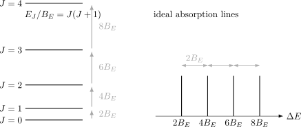
Ideal rigid-rotor levels obey $E_J=B_EJ(J+1)$. Electric-dipole transitions with $\Delta J=+1$ produce absorption lines at $\Delta E=2B_E,4B_E,6B_E,\ldots$, so the lines are equally spaced even though the level energies are quadratic in $J$.

Why a Permanent Dipole Matters

Pure rotational electric-dipole radiation couples through the molecular dipole operator. A linear molecule must have a permanent electric dipole in its body-fixed frame to show an ordinary microwave pure rotational spectrum.

This excludes ideal homonuclear diatomic molecules such as $\mathrm{H}_2$, $\mathrm{N}_2$, and $\mathrm{O}_2$ from the simplest electric-dipole pure rotational spectrum. They still have rotational energy levels, but the leading electric-dipole rotational transition is absent. Other mechanisms, Raman transitions, magnetic effects, collisions, and vibrational or electronic couplings are separate topics.

For a polar linear molecule, the dipole operator transforms as a vector under rotations. A vector operator carries angular momentum rank $1$, so angular-momentum addition permits

$$J' = J-1,\quad J,\quad J+1.$$

For pure rotational electric-dipole transitions between states of the same rotational band, the $J'=J$ case is excluded by the angular integral and parity structure, leaving

$$\Delta J=\pm1.$$

The allowed changes in $M$ depend on the radiation polarization and the chosen quantization axis:

$$\Delta M=0,\pm1.$$

In many first spectra the $M$ sublevels are unresolved, so one observes a line associated with the $J\to J+1$ transition rather than separate components for each $M$ value.

What Line Positions Measure

The line spacing gives the moment of inertia. If wavenumber line positions are ideal and adjacent lines are separated by

$$\Delta\tilde\nu_{\mathrm{line}} = 2\tilde B,$$

then

$$I = \frac{h}{8\pi^2c\tilde B} = \frac{h}{4\pi^2c\,\Delta\tilde\nu_{\mathrm{line}}}.$$

For a diatomic molecule this implies

$$R_e = \sqrt{\frac{I}{\mu}}.$$

This is the basic structural lesson of rotational spectroscopy: the spectrum is a ruler for moment of inertia. It does not by itself determine a full molecular geometry for a complicated molecule, but for a diatomic it directly constrains the bond length once the isotopic masses are known.

Isotopic substitution illustrates the same point. If the bond length is nearly unchanged but $\mu$ increases, then $I$ increases and $\tilde B$ decreases. The spectrum shifts toward smaller wavenumbers.

Intensities Are a Separate Question

Line positions come from energy differences. Line intensities also depend on populations and matrix elements.

At temperature $T$, the population of a rotational level is approximately proportional to

$$N_J \propto (2J+1) \exp\left[-\frac{B_EJ(J+1)}{k_BT}\right],$$

before including nuclear-spin statistical weights and other molecular details. The factor $2J+1$ is the degeneracy in $M$, while the exponential suppresses high $J$ at low temperature.

The transition strength also contains a dipole matrix element. The tensor-operator derivation of the rotor selection rule is in Applications to Molecular Rotations. A compact transition-rate treatment uses Fermi’s Golden Rule and the symmetry constraints summarized in Selection Rules and Transition Rates. This page only separates the first lesson:

$$\text{line position} \leftarrow \text{energy difference}, \qquad \text{line intensity} \leftarrow \text{population and matrix element}.$$

Corrections to the Ideal Ladder

Real rotational spectra are close to, but not exactly, the rigid-rotor ladder. Common corrections include:

• centrifugal distortion, because a rotating molecule stretches slightly at larger $J$;
• vibration-rotation coupling, because the average bond length depends on vibrational state;
• non-rigid and asymmetric-top effects in polyatomic molecules;
• hyperfine, spin-rotation, and external-field splittings;
• nuclear exchange symmetry restrictions for identical nuclei.

The most common first correction in wavenumber units is written schematically as

$$\tilde E_J = \tilde B J(J+1) - D[J(J+1)]^2 \cdots,$$

which shifts the line positions to

$$\tilde\nu_{J\to J+1} = 2\tilde B(J+1) - 4D(J+1)^3 \cdots.$$

The correction grows with $J$, so high-$J$ lines are where deviations from equal spacing first become hard to ignore. In this volume, the ideal result is the main canonical-system lesson; detailed fitting is spectroscopy.

Common Mistakes

• Confusing level spacings with line spacings. The allowed neighboring transition energies form the observed line ladder.
• Treating $B$ as a magnetic field rather than a rotational constant.
• Forgetting that electric-dipole pure rotational spectra require a permanent dipole for the simplest mechanism.
• Expecting homonuclear diatomic molecules to show the same microwave pure rotational spectrum as polar molecules.
• Inferring intensities from energy levels alone. Populations, degeneracies, dipole matrix elements, and temperature matter.
• Applying the ideal rigid-rotor formula at high $J$ without checking centrifugal distortion.
• Using half-integer $J$ for an ordinary scalar linear rotor. The rotational quantum number here is integer.

Exercises

1. A polar linear molecule has $\tilde B=1.50\,\mathrm{cm}^{-1}$. Find the first three ideal pure rotational absorption line positions in wavenumber units.

Solution

The absorption lines are

$$\tilde\nu_{J\to J+1} = 2\tilde B(J+1).$$

For $J=0,1,2$,

$$\begin{aligned} \tilde\nu_{0\to1}&=2(1.50\,\mathrm{cm}^{-1})=3.00\,\mathrm{cm}^{-1},\\ \tilde\nu_{1\to2}&=4(1.50\,\mathrm{cm}^{-1})=6.00\,\mathrm{cm}^{-1},\\ \tilde\nu_{2\to3}&=6(1.50\,\mathrm{cm}^{-1})=9.00\,\mathrm{cm}^{-1}. \end{aligned}$$

2. Derive the wavenumber rotational constant $\tilde B=h/(8\pi^2cI)$ from $E_J=\hbar^2J(J+1)/(2I)$.

Solution

By definition,

$$\tilde E_J = \frac{E_J}{hc} = \tilde B J(J+1).$$

Using

$$E_J = \frac{\hbar^2}{2I}J(J+1) = \frac{h^2}{8\pi^2I}J(J+1),$$

we get

$$\tilde B = \frac{1}{hc}\frac{h^2}{8\pi^2I} = \frac{h}{8\pi^2cI}.$$

3. If isotopic substitution doubles the reduced mass while leaving $R_e$ nearly fixed, what happens to $\tilde B$ and to the line spacing?

Solution

For a diatomic molecule,

$$I=\mu R_e^2.$$

If $\mu$ doubles and $R_e$ is unchanged, then $I$ doubles. Since

$$\tilde B = \frac{h}{8\pi^2cI},$$

$\tilde B$ is divided by $2$. The ideal adjacent line spacing is $2\tilde B$, so it is also divided by $2$.

4. Why does the absence of a permanent dipole not mean that a homonuclear diatomic molecule has no rotational levels?

Solution

The rotational levels come from the molecular kinetic-energy Hamiltonian:

$$E_J = \frac{\hbar^2}{2I}J(J+1).$$

The permanent dipole condition is a statement about the leading electric-dipole coupling to radiation. A homonuclear diatomic molecule can have rotational energy levels while lacking the simplest electric-dipole pure rotational transition. Energy levels and allowed radiative transitions are distinct questions.

Where This Is Used

• Rigid Rotor derives the underlying angular spectrum.
• Rotations of Molecules develops the semirigid molecular application beyond the ideal first encounter.
• Rovibrational Coupling develops branch-resolved vibration–rotation bands and their leading coupling corrections.
• Rigid Rotor as an Angular-Momentum System explains the $J(J+1)$ energy law as a rotational-Casimir result.
• Dynamical Symmetry explains the Casimir-operator viewpoint behind spectra such as $E_J\propto J(J+1)$.
• Particle on a Sphere gives the geometry-first version of the same eigenvalue problem.
• Spherical Harmonics as Wavefunctions explains how the angular eigenfunctions become probability amplitudes on the sphere.
• Rotor in External Fields: First Encounter previews Stark and Zeeman-style shifts of the ideal line ladder.
• Angular Momentum Algebra explains the integer $J,M$ labels and multiplet counting.
• Selection Rules and Transition Rates gives the broader symmetry language behind allowed and forbidden transitions.
• Selection Rule Problems includes solved rigid-rotor and electric-dipole selection-rule checks.
• Wigner D-Matrices are the natural mathematical language for full molecular orientations beyond this first linear-rotor treatment.

References

• G. Herzberg, Molecular Spectra and Molecular Structure I: Spectra of Diatomic Molecules, 2nd ed., Van Nostrand, 1950.
• C. H. Townes and A. L. Schawlow, Microwave Spectroscopy, Dover, 1975.
• R. N. Zare, Angular Momentum: Understanding Spatial Aspects in Chemistry and Physics, Wiley, 1988.
• P. W. Atkins and R. S. Friedman, Molecular Quantum Mechanics, 5th ed., Oxford University Press, 2011.
• B. H. Bransden and C. J. Joachain, Physics of Atoms and Molecules, 2nd ed., Pearson, 2003.