Spherical Harmonics as Wavefunctions

Spherical harmonics can be read in two complementary ways. Mathematically, they are an orthonormal basis for functions on the sphere. Physically, they are angular probability amplitudes: if a particle’s only configuration variable is direction, then a normalized spherical harmonic is a wavefunction on $S^2$.

This page explains that wavefunction interpretation. It focuses on probability density, angular nodes, real and complex bases, and visualization cautions. The formula definitions and phase conventions live in Spherical Harmonics, while the angular-momentum operator interpretation lives in Spherical Harmonics as Angular-Momentum States.

Wavefunctions on the Sphere

For a particle constrained to a sphere, the wavefunction is a complex function of direction:

$$\Psi(\Omega)=\Psi(\theta,\phi), \qquad \Omega\in S^2.$$

The probability density per unit solid angle is

$$\rho(\Omega)=\lvert\Psi(\Omega)\rvert^2.$$

Probabilities are computed with the sphere measure:

$$dP = \lvert\Psi(\theta,\phi)\rvert^2 \sin\theta\,d\theta\,d\phi = \lvert\Psi(\Omega)\rvert^2d\Omega.$$

Thus $\lvert\Psi\rvert^2$ is density per unit solid angle, not density per unit $\theta\,d\phi$. The factor $\sin\theta$ matters whenever one integrates over polar angle.

Normalization and Orthogonality

The normalized spherical harmonics obey

$$\int_{S^2} \lvert Y_\ell^m(\Omega)\rvert^2\,d\Omega =1.$$

More generally,

$$\int_{S^2} \left(Y_\ell^m\right)^* Y_{\ell'}^{m'}\,d\Omega = \delta_{\ell\ell'}\delta_{mm'}.$$

For fixed $\ell$, the integer $m$ runs from $-\ell$ to $\ell$, giving $2\ell+1$ orthonormal angular states. A general square-integrable angular wavefunction can be expanded as

$$\Psi(\Omega) = \sum_{\ell=0}^\infty \sum_{m=-\ell}^{\ell} c_{\ell m}Y_\ell^m(\Omega).$$

The coefficients are probability amplitudes for angular-momentum basis states:

$$c_{\ell m} = \int_{S^2} \left(Y_\ell^m\right)^* \Psi\,d\Omega.$$

Angular Density and Marginals

The full angular density is $\lvert Y_\ell^m(\theta,\phi)\rvert^2$ per unit solid angle. If one asks for a probability distribution in polar angle alone, the azimuth must be integrated out:

$$p(\theta) = \int_0^{2\pi} \lvert Y_\ell^m(\theta,\phi)\rvert^2 \sin\theta\,d\phi.$$

This distinction is a common source of visual mistakes. A plot of $\lvert Y\rvert^2$ against $\theta$ is not automatically a polar-angle probability distribution unless the $\sin\theta$ measure has been included.

For $Y_0^0=1/\sqrt{4\pi}$, the density per solid angle is constant:

$$\lvert Y_0^0\rvert^2=\frac{1}{4\pi}.$$

But the marginal polar distribution is

$$p(\theta) = \frac{1}{2}\sin\theta.$$

There is more area near the equator than near either pole.

Angular Nodes

An angular node is a set of directions where the angular wavefunction vanishes. Nodes are properties of the amplitude, not of the probability density alone.

For example,

$$Y_1^0(\theta,\phi) \propto \cos\theta.$$

It vanishes at

$$\theta=\frac{\pi}{2},$$

so its angular node is the equator. The probability density has two lobes, one in the northern hemisphere and one in the southern hemisphere, but the sign or phase of the amplitude changes across the node.

For complex $Y_\ell^m$, the factor $e^{im\phi}$ changes phase around the $z$ axis. It does not by itself create $\phi$-dependent zeros, because its magnitude is $1$. Real linear combinations can have nodal meridian planes that are easier to draw.

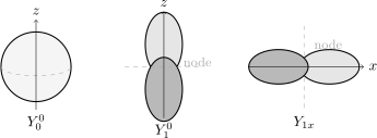
Schematic angular shapes. Shading distinguishes sign or phase of the angular amplitude; probabilities are computed from $\lvert Y\rvert^2d\Omega$. The dashed sets indicate angular nodes.

Real and Complex Bases

The standard $Y_\ell^m$ are complex eigenfunctions of both $\hat L^2$ and $\hat L_z$:

$$\hat L^2Y_\ell^m = \hbar^2\ell(\ell+1)Y_\ell^m, \qquad \hat L_zY_\ell^m = \hbar mY_\ell^m.$$

They are the natural basis when a $z$ axis and $L_z$ measurement are part of the problem.

Real spherical harmonics are linear combinations inside the same fixed-$\ell$ subspace. For the $\ell=1$ sector, a common convention is

$$Y_{1z}=Y_1^0, \qquad Y_{1x}\propto \frac{Y_1^{-1}-Y_1^1}{\sqrt{2}}, \qquad Y_{1y}\propto \frac{i(Y_1^{-1}+Y_1^1)}{\sqrt{2}}.$$

Overall phases and signs depend on convention. The important point is basis-invariant: $Y_{1x}$, $Y_{1y}$, and $Y_{1z}$ span the same $\ell=1$ angular subspace as $Y_1^{-1}$, $Y_1^0$, and $Y_1^1$.

Real harmonics are often better for drawing nodal planes and lobes. Complex harmonics are better for definite $L_z$ and phase winding. Neither basis is more physical without a question that selects which observables are being emphasized.

Visualization Cautions

Spherical-harmonic pictures are useful, but the plotting convention must be stated. Common conventions include:

• plotting radius proportional to $\lvert Y(\Omega)\rvert$;
• plotting radius proportional to $\lvert Y(\Omega)\rvert^2$;
• coloring a surface by sign, phase, or real part;
• drawing only nodal curves on a unit sphere;
• drawing real harmonics even when the eigenbasis being discussed is complex.

These conventions answer different visual questions. A lobe drawing is not a literal surface where the particle lives. The particle’s configuration space is already the sphere; the drawing is a way to encode amplitude or probability on that sphere.

For complex harmonics with $m\ne0$, a two-color positive/negative lobe picture is usually inadequate because the phase varies continuously. Phase-color plots or separate real and imaginary parts are more honest.

Relation to Atomic Orbitals

In central-potential problems, a full wavefunction has the separated form

$$\psi(r,\theta,\phi) = R(r)Y_\ell^m(\theta,\phi).$$

The spherical harmonic is only the angular factor. It determines angular nodes and angular momentum labels, but it does not determine radial nodes, radial size, or radial probability. Those belong to the radial wavefunction.

This is why Atomic Orbitals need both spherical harmonics and radial functions. Orbital pictures often mix both ingredients into one three-dimensional visualization.

Common Mistakes

• Forgetting that probabilities use $d\Omega=\sin\theta\,d\theta\,d\phi$.
• Treating $\lvert Y\rvert^2$ as a density per unit $\theta$ instead of per unit solid angle.
• Confusing a spherical harmonic with a full hydrogenic orbital.
• Assuming a real lobe drawing represents an $\hat L_z$ eigenstate.
• Interpreting colors as electric charge rather than sign or phase.
• Forgetting that complex spherical harmonics have phase winding, not just positive and negative lobes.
• Treating coordinate singularities at the poles as physical nodes.

Exercises

1. Find the polar-angle marginal distribution for $Y_0^0$.

Solution

Since

$$Y_0^0=\frac{1}{\sqrt{4\pi}},$$

we have

$$\lvert Y_0^0\rvert^2=\frac{1}{4\pi}.$$

The polar marginal is

$$p(\theta) = \int_0^{2\pi} \frac{1}{4\pi} \sin\theta\,d\phi = \frac{1}{2}\sin\theta.$$

2. Show that $Y_1^0$ has an equatorial angular node.

Solution

Up to normalization,

$$Y_1^0(\theta,\phi)\propto\cos\theta.$$

The zero occurs when

$$\cos\theta=0,$$

which gives

$$\theta=\frac{\pi}{2}.$$

That is the equator of the sphere.

3. Why is a real $Y_{1x}$-type harmonic not an $\hat L_z$ eigenstate?

Solution

A real $Y_{1x}$-type harmonic is a linear combination of $m=-1$ and $m=1$ states:

$$Y_{1x}\propto \frac{Y_1^{-1}-Y_1^1}{\sqrt{2}}.$$

The two components have different $\hat L_z$ eigenvalues, $-\hbar$ and $+\hbar$. Applying $\hat L_z$ therefore does not return a single constant times $Y_{1x}$. It remains a valid member of the $\ell=1$ subspace, but it is not an $\hat L_z$ eigenfunction.

4. Explain why $\lvert Y_\ell^m\rvert^2$ for complex $Y_\ell^m$ is independent of $\phi$ when only the factor $e^{im\phi}$ carries the azimuthal dependence.

Solution

The azimuthal factor has unit magnitude:

$$\left\lvert e^{im\phi}\right\rvert^2=1.$$

Therefore it contributes phase but not magnitude. The probability density for a single complex $Y_\ell^m$ depends on $\phi$ only if another part of the angular function carries $\phi$ dependence, which the standard separated spherical harmonic does not. Real combinations of different $m$ values can have $\phi$-dependent densities.

Where This Is Used

• Particle on a Sphere uses spherical harmonics as the full energy eigenfunctions.
• Rigid Rotor uses the same functions for molecular orientation.
• Angular Probability Distributions gives the general measure and marginal-distribution rules used here.
• Angular and Radial Separation uses spherical harmonics as the universal angular factors in central potentials.
• Atomic Orbitals combines these angular functions with radial wavefunctions.
• Spherical Harmonics is the mathematical reference for normalization, phase conventions, and completeness.
• Spherical Harmonics as Angular-Momentum States gives the operator interpretation.

References

• D. J. Griffiths and D. F. Schroeter, Introduction to Quantum Mechanics, 3rd ed., Cambridge University Press, 2018.
• R. Shankar, Principles of Quantum Mechanics, 2nd ed., Springer, 1994.
• J. J. Sakurai and J. Napolitano, Modern Quantum Mechanics, 3rd ed., Cambridge University Press, 2020.
• A. R. Edmonds, Angular Momentum in Quantum Mechanics, Princeton University Press, 1957.
• R. N. Zare, Angular Momentum: Understanding Spatial Aspects in Chemistry and Physics, Wiley, 1988.