Rotor in External Fields: First Encounter

An isolated rigid rotor has full rotational symmetry. Its energy depends on $J$ but not on $M$, so every level with $J\gt0$ contains a $(2J+1)$-fold multiplet. An external field changes the question: the field selects a direction in space, breaks the full rotational symmetry, and can split or mix states that were previously degenerate.

This page is a first encounter. It explains the symmetry logic and the simplest electric-field coupling for a polar linear rotor. Detailed Stark and Zeeman spectroscopy, line strengths in fields, hyperfine structure, and molecular-structure fits belong to later molecular and approximation-method pages.

Field-Free Starting Point

The ideal linear rotor Hamiltonian is

$$\hat H_0 = B_E\hat J^2/\hbar^2, \qquad B_E = \frac{\hbar^2}{2I}.$$

The eigenstates are

$$\lvert J,M\rangle, \qquad J=0,1,2,\ldots, \qquad M=-J,\ldots,J,$$

with energies

$$E_J^{(0)} = B_EJ(J+1).$$

The energy does not depend on $M$. The degeneracy is a symmetry statement: without a selected axis, the different orientations of a fixed angular-momentum multiplet are physically equivalent.

What an External Field Does

A static uniform field supplies a laboratory vector. If the field is chosen along the lab $z$ axis, the full rotation symmetry is reduced to rotations about that axis:

$$SO(3) \longrightarrow SO(2).$$

The usual consequence is:

• $M$ often remains a good quantum number, because rotations about the field axis remain a symmetry.
• $J$ need not remain a good quantum number, because the field can mix different total-angular-momentum multiplets.
• The old $M$ degeneracy can be partly or fully lifted.
• Parity can be broken by a static electric field acting on a permanent dipole.

The exact outcome depends on the coupling. A scalar perturbation preserves more symmetry than a vector perturbation; a magnetic field can also break time-reversal symmetry.

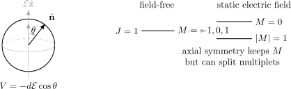
A static electric field selects the lab $z$ axis. For a polar rotor, the interaction $V=-d\mathcal E\cos\theta$ depends on the angle between the molecular axis and the field. Axial symmetry can preserve $M$ while splitting the field-free $M$ multiplet.

Polar Rotor in a Static Electric Field

For a polar linear molecule with body-fixed dipole magnitude $d$, a static electric field

$$\boldsymbol{\mathcal E} = \mathcal E\hat{\mathbf z}$$

gives the orienting interaction

$$\hat V_E = - \mathbf d\cdot\boldsymbol{\mathcal E} = - d\mathcal E\cos\theta,$$

where $\theta$ is the angle between the molecular axis and the field axis.

The Hamiltonian is

$$\hat H = B_E\hat J^2/\hbar^2 - d\mathcal E\cos\theta.$$

The dimensionless field strength is roughly

$$\eta = \frac{d\mathcal E}{B_E}.$$

When $\eta\ll1$, perturbation theory is appropriate. When $\eta$ is large, the rotor becomes partially oriented and the eigenstates are often called pendular states. That strong-field regime is beyond this first encounter.

Why the Electric Field Mixes J

The operator $\cos\theta$ is not diagonal in $J$. Its action on spherical harmonics has the form

$$\cos\theta\,Y_J^M = a_{J+1,M}Y_{J+1}^M + a_{J,M}Y_{J-1}^M,$$

where

$$a_{J+1,M} = \sqrt{ \frac{(J+1)^2-M^2} {(2J+1)(2J+3)} },$$

and

$$a_{J,M} = \sqrt{ \frac{J^2-M^2} {(2J-1)(2J+1)} }.$$

Thus the static electric field couples states with

$$\Delta J=\pm1, \qquad \Delta M=0$$

when the field defines the lab $z$ axis. The $M$ selection rule is the axial-symmetry statement. The $\Delta J$ rule is the angular structure of a vector operator.

Weak-Field Stark Lesson

For the simple linear rigid rotor, the diagonal matrix element

$$\langle J,M\vert\cos\theta\vert J,M\rangle$$

vanishes. One way to see this is parity: $\lvert J,M\rangle$ has parity $(-1)^J$, while $\cos\theta$ is parity odd. Therefore the first-order Stark shift is zero for an isolated field-free rotor level.

The first nonzero shift is typically second order in the electric field. For the ground state, only $\lvert1,0\rangle$ contributes at lowest order because

$$\cos\theta\,Y_0^0 = \frac{1}{\sqrt3}Y_1^0.$$

Using

$$E_1^{(0)}-E_0^{(0)} = 2B_E,$$

the second-order shift is

$$\begin{aligned} \Delta E_{0,0}^{(2)} &= \frac{ \left\lvert \langle1,0\vert (-d\mathcal E\cos\theta) \vert0,0\rangle \right\rvert^2 } {E_0^{(0)}-E_1^{(0)}} \\ &= - \frac{d^2\mathcal E^2}{6B_E}. \end{aligned}$$

This negative shift is the simplest quantum version of induced alignment: the field lowers the energy by admixing a small amount of the $J=1$ state into the $J=0$ ground state.

Degeneracy Breaking

The field-free rotor has energy $E_J^{(0)}$ independent of $M$. A static electric field along $z$ preserves rotations about $z$, so $M$ remains a useful label, but the energy shifts can depend on $M$.

For an electric field alone and no additional time-reversal breaking, states with $M$ and $-M$ often remain degenerate. Thus the $J=1$ triplet can split into an $M=0$ level and a twofold $\lvert M\rvert=1$ level rather than three unrelated levels.

A magnetic field can split the signs of $M$ if the rotor has a magnetic moment that couples to the field. In a simple effective model with

$$\boldsymbol\mu = \gamma\hat{\mathbf J},$$

the Zeeman-like perturbation is

$$\hat V_B = - \boldsymbol\mu\cdot\mathbf B = - \gamma B_z\hat J_z.$$

Then

$$\Delta E_{J,M}^{(1)} = - \gamma B_z\hbar M.$$

This formula is a model for a rotor with the stated magnetic moment. It should not be applied automatically to every neutral rigid rotor.

Good Quantum Numbers in a Field

The safest way to decide labels is to ask what commutes with the Hamiltonian.

For the field-free rotor,

$$[\hat H_0,\hat J^2]=0, \qquad [\hat H_0,\hat J_z]=0.$$

For the electric-field rotor,

$$\hat H = B_E\hat J^2/\hbar^2 - d\mathcal E\cos\theta,$$

the Hamiltonian still commutes with $\hat J_z$:

$$[\hat H,\hat J_z]=0,$$

because the field is axially symmetric about $z$. But it does not commute with $\hat J^2$:

$$[\hat H,\hat J^2]\ne0.$$

Therefore $M$ can label exact eigenstates in the static field, while $J$ becomes an approximate or field-free label when the electric coupling is nonzero.

Relation to Spectroscopy

External fields change rotational spectra in two ways. First, they shift the energy levels. Second, they change the eigenstates, and therefore change transition matrix elements and selection-rule details.

In weak fields, one often speaks of Stark or Zeeman shifts of the field-free rotational lines. In stronger fields, the states are better described as field-dressed rotor states, and the field-free $J$ label becomes only a guide.

The canonical lesson here is modest but important: a degeneracy is not just a repeated number in a formula. It encodes a symmetry. Once an external field removes part of the symmetry, the degeneracy can split.

Common Mistakes

• Treating an external field as adding the same constant energy to every rotor state.
• Assuming $J$ remains an exact quantum number for a polar rotor in a static electric field.
• Expecting a first-order Stark shift for the $J=0$ state of a simple linear rotor.
• Forgetting that an electric field can preserve $M$ while mixing different $J$ values.
• Applying a permanent-dipole coupling to a homonuclear diatomic molecule with no body-fixed electric dipole.
• Using a Zeeman formula without specifying the magnetic moment that couples to the field.
• Confusing the lab field axis with the molecule’s body-fixed axis.

Exercises

1. Which field-free quantum numbers remain exact for a polar linear rotor in a static electric field along $z$?

Solution

The field leaves rotations about the $z$ axis as a symmetry, so $M$ remains exact. The perturbation is proportional to $\cos\theta$, which mixes $J$ with $J\pm1$, so $J$ is not exact once the field is nonzero.

2. Show directly that the first-order Stark shift of the $J=0$ state vanishes.

Solution

For $J=0$,

$$Y_0^0 = \frac{1}{\sqrt{4\pi}}.$$

The first-order shift is proportional to

$$\int_{S^2} \left(Y_0^0\right)^* \cos\theta Y_0^0\,d\Omega.$$

This is

$$\frac{1}{4\pi} \int_0^{2\pi} \int_0^\pi \cos\theta\sin\theta\,d\theta\,d\phi = 0,$$

because the integrand is odd under reflection across the equator.

3. Use $\cos\theta\,Y_0^0=Y_1^0/\sqrt3$ to compute the second-order ground-state Stark shift.

Solution

The only coupled state at this order is $\lvert1,0\rangle$. The matrix element is

$$\langle1,0\vert (-d\mathcal E\cos\theta) \vert0,0\rangle = - \frac{d\mathcal E}{\sqrt3}.$$

Since $E_1^{(0)}-E_0^{(0)}=2B_E$,

$$\Delta E_{0,0}^{(2)} = \frac{d^2\mathcal E^2/3}{-2B_E} = - \frac{d^2\mathcal E^2}{6B_E}.$$

4. In the effective magnetic model $\hat V_B=-\gamma B_z\hat J_z$, what are the first-order shifts of the $J=1$ states?

Solution

For $J=1$, the possible values are

$$M=-1,0,1.$$

Since $\hat J_z\lvert J,M\rangle=\hbar M\lvert J,M\rangle$,

$$\Delta E_{1,M}^{(1)} = - \gamma B_z\hbar M.$$

Thus

$$\Delta E_{1,-1}^{(1)} = \gamma B_z\hbar, \qquad \Delta E_{1,0}^{(1)} = 0, \qquad \Delta E_{1,1}^{(1)} = - \gamma B_z\hbar.$$

Where This Is Used

• Rigid Rotor gives the field-free spectrum and degeneracy.
• Rotational Spectra explains the ideal line ladder before fields shift or split levels.
• Angular Probability Distributions explains the angular measure used in matrix elements such as $\langle\cos\theta\rangle$.
• Symmetry Constraints on Hamiltonians gives the broader symmetry language for what a field can break.
• Nondegenerate Perturbation Theory supplies the weak-field expansion used for the $J=0$ Stark shift.
• Degenerate Perturbation Theory is needed when a perturbation acts inside an exactly degenerate subspace.
• Minimal Coupling in Wave Mechanics treats electromagnetic potentials for charged particles, a different but related way fields enter Hamiltonians.

References

• R. N. Zare, Angular Momentum: Understanding Spatial Aspects in Chemistry and Physics, Wiley, 1988.
• G. Herzberg, Molecular Spectra and Molecular Structure I: Spectra of Diatomic Molecules, 2nd ed., Van Nostrand, 1950.
• C. H. Townes and A. L. Schawlow, Microwave Spectroscopy, Dover, 1975.
• P. W. Atkins and R. S. Friedman, Molecular Quantum Mechanics, 5th ed., Oxford University Press, 2011.
• D. J. Griffiths and D. F. Schroeter, Introduction to Quantum Mechanics, 3rd ed., Cambridge University Press, 2018.