Angular Probability Distributions

Angular wavefunctions become probability distributions only after the measure is specified. On a circle, the natural measure is the angle element $d\theta$. On a sphere, the natural measure is the solid-angle element

$$d\Omega = \sin\theta\,d\theta\,d\phi.$$

The extra factor $\sin\theta$ is not a normalization detail. It expresses the geometry of the sphere: equal changes in polar angle do not sweep out equal areas.

This page is the measure-first companion to Particle on a Ring, Particle on a Sphere, and Spherical Harmonics as Wavefunctions. It explains how to turn angular amplitudes into probabilities, marginals, and plots without quietly changing the measure.

Densities Need Measures

A density is not a probability by itself. It is a function integrated against a measure:

$$P(A) = \int_A \rho\,d\mu.$$

For angular variables, two functions can look different but represent the same distribution if they are densities with respect to different measures. The phrase “density per unit angle” is not the same as “density per unit solid angle.”

In quantum mechanics, a normalized wavefunction on configuration space gives

$$dP = \lvert\psi\rvert^2\,d\mu.$$

The measure $d\mu$ belongs to the configuration space, not to personal convention. For a ring it is $d\theta$; for a sphere it is $d\Omega$.

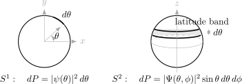
On $S^1$, probability is naturally density per unit angle. On $S^2$, probability is naturally density per unit solid angle, so a coordinate rectangle contributes the geometric factor $\sin\theta$.

Probability on a Circle

For a particle on a ring, the coordinate is one angle:

$$0\le\theta\lt2\pi, \qquad \theta\sim\theta+2\pi.$$

The Hilbert space is $L^2(S^1,d\theta)$, and a normalized wavefunction satisfies

$$\int_0^{2\pi} \lvert\psi(\theta)\rvert^2\,d\theta = 1.$$

The probability of finding the particle in an angular interval $A$ is

$$P(A) = \int_A \lvert\psi(\theta)\rvert^2\,d\theta.$$

Thus $\lvert\psi(\theta)\rvert^2$ is density per unit angle. If one uses arc length $s=R\theta$ instead, then $ds=R\,d\theta$, and the density per unit length is

$$\rho_s(s) = \frac{1}{R} \left\lvert \psi\left(\frac{s}{R}\right) \right\rvert^2.$$

Both descriptions give the same probabilities when the measure is included.

For the normalized angular-momentum eigenstate

$$u_m(\theta) = \frac{1}{\sqrt{2\pi}}e^{im\theta},$$

the density is uniform:

$$\lvert u_m(\theta)\rvert^2 = \frac{1}{2\pi}.$$

The probability in an interval of angular width $\Delta\theta$ is $\Delta\theta/(2\pi)$.

Probability on a Sphere

For a particle constrained to a sphere, or for a linear rotor orientation, the configuration space is $S^2$. A wavefunction is a function of direction,

$$\Psi(\Omega) = \Psi(\theta,\phi),$$

and the natural measure is

$$d\Omega = \sin\theta\,d\theta\,d\phi.$$

Normalization is

$$\int_0^{2\pi} \int_0^\pi \lvert\Psi(\theta,\phi)\rvert^2 \sin\theta\,d\theta\,d\phi = 1.$$

The probability of an angular region $A\subset S^2$ is

$$P(A) = \int_A \lvert\Psi(\Omega)\rvert^2\,d\Omega.$$

Thus $\lvert\Psi(\Omega)\rvert^2$ is density per unit solid angle. If one instead wants a density with respect to the coordinate area $d\theta\,d\phi$, it is

$$\rho_{\theta\phi}(\theta,\phi) = \lvert\Psi(\theta,\phi)\rvert^2\sin\theta.$$

This is the same probability distribution written with a different reference measure.

Where the Sine Factor Comes From

On a sphere of radius $R$, a small displacement in the polar direction has length $R\,d\theta$. A small displacement in the azimuthal direction at polar angle $\theta$ has length

$$R\sin\theta\,d\phi.$$

The corresponding area element is therefore

$$dA = R^2\sin\theta\,d\theta\,d\phi.$$

Dividing by $R^2$ gives the solid-angle element $d\Omega$. Near the poles, circles of constant $\theta$ are small. Near the equator, they are large. That is the geometric content of $\sin\theta$.

For a full latitude band between $\theta$ and $\theta+d\theta$,

$$d\Omega_{\mathrm{band}} = 2\pi\sin\theta\,d\theta.$$

This band has very little area near $\theta=0$ or $\theta=\pi$, and maximal area near $\theta=\pi/2$.

Marginal Angular Distributions

The full angular density on the sphere is a density per unit solid angle. If one asks only for the polar-angle distribution, the azimuth must be integrated out:

$$p_\theta(\theta) = \int_0^{2\pi} \lvert\Psi(\theta,\phi)\rvert^2 \sin\theta\,d\phi.$$

This is a one-dimensional density with respect to $d\theta$:

$$\int_0^\pi p_\theta(\theta)\,d\theta = 1.$$

Similarly, the azimuthal marginal is

$$p_\phi(\phi) = \int_0^\pi \lvert\Psi(\theta,\phi)\rvert^2 \sin\theta\,d\theta,$$

with

$$\int_0^{2\pi} p_\phi(\phi)\,d\phi = 1.$$

For the constant angular wavefunction

$$\Psi_0 = \frac{1}{\sqrt{4\pi}},$$

the density per unit solid angle is constant:

$$\lvert\Psi_0\rvert^2 = \frac{1}{4\pi}.$$

But the polar-angle marginal is not constant:

$$p_\theta(\theta) = \int_0^{2\pi} \frac{1}{4\pi} \sin\theta\,d\phi = \frac{1}{2}\sin\theta.$$

An isotropic direction is uniform on the sphere, not uniform in the coordinate $\theta$.

Uniform in Direction Means Uniform in Cosine

The clean coordinate for polar-angle sampling is

$$u=\cos\theta.$$

Since

$$du=-\sin\theta\,d\theta,$$

the solid-angle element becomes

$$d\Omega = d\phi\,(-du).$$

Ignoring the orientation sign in the integration limits, this means that the uniform distribution on the sphere is uniform in $u=\cos\theta$ and in $\phi$, not uniform in $\theta$ and $\phi$.

For an isotropic state,

$$p_u(u) = \frac{1}{2}, \qquad -1\le u\le1.$$

This is why equal bins in $\cos\theta$ correspond to equal-area polar bands, while equal bins in $\theta$ do not.

Example: The Y One Zero State

The spherical harmonic $Y_1^0$ is proportional to $\cos\theta$:

$$Y_1^0(\theta,\phi) = \sqrt{\frac{3}{4\pi}}\cos\theta.$$

Its density per unit solid angle is

$$\lvert Y_1^0\rvert^2 = \frac{3}{4\pi}\cos^2\theta.$$

The polar-angle marginal is

$$\begin{aligned} p_\theta(\theta) &= \int_0^{2\pi} \frac{3}{4\pi}\cos^2\theta \sin\theta\,d\phi \\ &= \frac{3}{2}\cos^2\theta\,\sin\theta. \end{aligned}$$

The factor $\cos^2\theta$ comes from the amplitude. The factor $\sin\theta$ comes from the sphere. A correct polar plot of probability versus $\theta$ must include both.

Visualization Cautions

Angular plots often hide the measure. The following distinctions should be kept explicit:

• A heat map of $\lvert\Psi(\theta,\phi)\rvert^2$ on a rectangular $\theta,\phi$ grid is not an equal-area map of the sphere.
• A plot of $\lvert\Psi\rvert^2$ versus $\theta$ is not the polar-angle marginal unless the $\sin\theta$ factor and the $\phi$ integral are included.
• Equal-width bins in $\theta$ do not have equal solid angle.
• Color on an orbital or spherical-harmonic plot may represent sign or phase, not probability.
• A lobe surface may show amplitude magnitude, probability density, or a chosen isosurface. Read the caption before interpreting it.
• The poles are coordinate singularities for $\phi$, not physical points with many distinct azimuthal states.

For numerical work, equal-area integration is usually easiest if the grid or quadrature weights explicitly include $\sin\theta$, or if the polar coordinate is changed to $u=\cos\theta$.

Common Mistakes

• Calling $\lvert\Psi(\theta,\phi)\rvert^2$ a density per unit $\theta\,d\phi$ instead of per unit solid angle.
• Sampling $\theta$ uniformly when the intended distribution is uniform over directions.
• Forgetting that a small cap near the pole contains less area than a band of the same $\Delta\theta$ near the equator.
• Comparing angular plots without checking whether they show amplitude, density per solid angle, or a marginal density.
• Normalizing a spherical wavefunction with $d\theta\,d\phi$ instead of $\sin\theta\,d\theta\,d\phi$.
• Treating a coordinate singularity at the pole as a physical probability enhancement.

Exercises

1. A particle on a ring is in $u_m(\theta)=e^{im\theta}/\sqrt{2\pi}$. What is the probability of finding it in an interval of angular width $\Delta\theta$?

Solution

The density is

$$\lvert u_m(\theta)\rvert^2 = \frac{1}{2\pi}.$$

Therefore an interval of width $\Delta\theta$ has probability

$$P = \int_{\mathrm{interval}} \frac{1}{2\pi}\,d\theta = \frac{\Delta\theta}{2\pi}.$$

2. For an isotropic distribution on the sphere, compute the probability inside the polar cap $0\le\theta\le\theta_0$.

Solution

For an isotropic distribution,

$$\lvert\Psi\rvert^2 = \frac{1}{4\pi}.$$

Thus

$$\begin{aligned} P(0\le\theta\le\theta_0) &= \int_0^{2\pi} \int_0^{\theta_0} \frac{1}{4\pi} \sin\theta\,d\theta\,d\phi \\ &= \frac{1}{2} \int_0^{\theta_0}\sin\theta\,d\theta \\ &= \frac{1-\cos\theta_0}{2}. \end{aligned}$$

3. Check that the polar marginal for $Y_1^0$ is normalized.

Solution

The marginal is

$$p_\theta(\theta) = \frac{3}{2}\cos^2\theta\,\sin\theta.$$

Then

$$\int_0^\pi p_\theta(\theta)\,d\theta = \frac{3}{2} \int_0^\pi \cos^2\theta\,\sin\theta\,d\theta.$$

Let $u=\cos\theta$, so $du=-\sin\theta\,d\theta$. The limits change from $u=1$ to $u=-1$:

$$\frac{3}{2} \int_{-1}^{1} u^2\,du = \frac{3}{2} \frac{2}{3} = 1.$$

4. A simulation wants directions uniformly distributed on the sphere. Should it sample $\theta$ uniformly from $0$ to $\pi$?

Solution

No. Uniform $\theta$ overweights directions near the poles relative to the sphere’s area measure. A uniform direction can be generated by sampling

$$u=\cos\theta$$

uniformly from $-1$ to $1$, and sampling $\phi$ uniformly from $0$ to $2\pi$. Then $\theta=\arccos u$.

Where This Is Used

• Particle on a Ring uses $d\theta$ as the probability measure on $S^1$.
• Particle on a Sphere uses $d\Omega$ as the probability measure on $S^2$.
• Spherical Harmonics as Wavefunctions applies these rules to $Y_\ell^m$ states.
• Rigid Rotor uses the same angular measure for molecular orientations.
• Spherical Coordinates derives the coordinate measure inside three-dimensional wave mechanics.
• Normalization Table gives a quick lookup for angular, radial, box, continuum, and grid normalizations.
• Probability Densities gives the general mathematical rule that densities are defined relative to a measure.

References

• D. J. Griffiths and D. F. Schroeter, Introduction to Quantum Mechanics, 3rd ed., Cambridge University Press, 2018.
• R. Shankar, Principles of Quantum Mechanics, 2nd ed., Springer, 1994.
• G. B. Arfken, H. J. Weber, and F. E. Harris, Mathematical Methods for Physicists, 7th ed., Academic Press, 2013.
• R. N. Zare, Angular Momentum: Understanding Spatial Aspects in Chemistry and Physics, Wiley, 1988.