Atomic Orbitals

An atomic orbital is a one-electron wavefunction used to describe the spatial state of an electron bound to a nucleus. In the exact nonrelativistic hydrogenic problem, orbitals are stationary eigenfunctions of the point-Coulomb Hamiltonian. In many-electron atoms and molecules, the same word is also used for approximate one-electron functions inside a larger many-body description.

This page treats the clean hydrogenic meaning. It explains the $s,p,d,\ldots$ notation, probability-density interpretation, real and complex orbital bases, nodal surfaces, and common visualization traps. Many-electron and chemical-orbital uses should be read as later applications of this one-electron prototype, not as part of the exact hydrogen solution.

Definition in the Hydrogenic Problem

For a spinless one-electron Coulomb problem, the bound-state wavefunctions separate as

$$\psi_{n\ell m}(r,\theta,\phi) = R_{n\ell}(r)Y_\ell^m(\theta,\phi).$$

The quantum numbers obey

$$n=1,2,\ldots, \qquad \ell=0,1,\ldots,n-1, \qquad m=-\ell,\ldots,\ell.$$

The radial factor $R_{n\ell}$ is described in Radial Wavefunctions. The angular factor is a spherical harmonic. Together they define a spatial orbital.

The shell-level angular organization of these labels is summarized in Hydrogen Atom Angular Structure.

An orbital is not a classical path. It is a wavefunction, and its physical probability density is

$$\rho_{n\ell m}(\mathbf r) = \lvert\psi_{n\ell m}(\mathbf r)\rvert^2 = \lvert R_{n\ell}(r)\rvert^2 \lvert Y_\ell^m(\theta,\phi)\rvert^2.$$

For the ideal Coulomb Hamiltonian, $\psi_{n\ell m}$ is stationary up to the phase factor $e^{-iE_nt/\hbar}$. The density $\lvert\psi\rvert^2$ is then time-independent.

s, p, d, f Notation

The spectroscopic letter names the orbital angular-momentum quantum number $\ell$.

Letter	$\ell$	Number of $m$ values	Angular character
$s$	$0$	$1$	spherical angular factor
$p$	$1$	$3$	one angular nodal surface in a real basis
$d$	$2$	$5$	two angular nodal surfaces in a real basis
$f$	$3$	$7$	three angular nodal surfaces in a real basis

The shell label combines $n$ with the letter. Thus $1s$ means $n=1,\ell=0$, $2p$ means $n=2,\ell=1$, and $3d$ means $n=3,\ell=2$. The $m$ label still matters: for example, the $2p$ subshell contains three independent spatial orbitals.

The number of spatial orbitals in a fixed $\ell$ subshell is

$$2\ell+1.$$

If electron spin is included without spin-dependent interactions, each spatial orbital can be paired with two spin states. The word orbital by itself usually refers only to the spatial wavefunction unless a spin-orbital convention has been explicitly introduced.

Probability Densities and Radial Probability

The three-dimensional probability for the electron to lie in a region $\Omega$ is

$$\int_\Omega \lvert\psi(\mathbf r)\rvert^2\,d^3r.$$

In spherical coordinates,

$$d^3r=r^2\sin\theta\,dr\,d\theta\,d\phi.$$

After integrating over angles, the radial probability density is

$$P_{n\ell}(r) = r^2\lvert R_{n\ell}(r)\rvert^2.$$

This radial density is not the same object as the full three-dimensional density. For example, the hydrogen $1s$ wavefunction is largest at $r=0$, but the radial probability density is maximal at one Bohr radius because of the $r^2$ volume factor.

Orbital pictures usually show an isosurface of $\lvert\psi\rvert^2$ or a surface enclosing a chosen probability such as 90 or 95 percent. The boundary in such a picture is a visualization convention, not a hard edge of the atom.

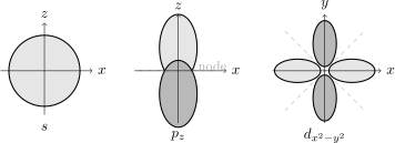
Schematic real-orbital shapes and nodal surfaces. The shaded lobes represent relative sign or phase of the wavefunction, not separate charged objects; probabilities come from $\lvert\psi\rvert^2$.

Real and Complex Orbitals

The separated functions $Y_\ell^m$ are complex angular-momentum eigenfunctions. They are simultaneous eigenfunctions of $\hat{\mathbf L}^2$ and $\hat L_z$:

$$\hat{\mathbf L}^2Y_\ell^m = \hbar^2\ell(\ell+1)Y_\ell^m, \qquad \hat L_zY_\ell^m = \hbar mY_\ell^m.$$

Complex orbitals are therefore natural when the $z$ component of angular momentum is being measured or when axial symmetry selects a preferred axis.

Real orbital pictures are different bases in the same degenerate $\ell$ subspace. For the $p$ orbitals, one common convention is

$$p_z\propto Y_1^0, \qquad p_x\propto \frac{Y_1^{-1}-Y_1^1}{\sqrt{2}}, \qquad p_y\propto \frac{i(Y_1^{-1}+Y_1^1)}{\sqrt{2}}.$$

Overall signs and phases depend on the spherical-harmonic convention, but the three-dimensional subspace is the same. The real orbitals $p_x,p_y,p_z$ are convenient for visualizing nodal planes and directional bonding. They are not all eigenstates of $\hat L_z$.

This distinction is harmless in the ideal hydrogenic problem because all $m$ states with fixed $n$ and $\ell$ are degenerate. A linear combination inside the degenerate subspace is still a stationary state. If an external magnetic field selects a $z$ axis, however, the complex $m$ eigenstates often become the better basis.

Nodal Surfaces

A node is a place where the wavefunction vanishes. Hydrogenic orbitals have radial nodes from $R_{n\ell}(r)$ and angular nodes from $Y_\ell^m(\theta,\phi)$ or from real linear combinations of spherical harmonics.

For hydrogenic bound states,

$$\text{number of radial nodes} = n-\ell-1.$$

The number of angular nodal surfaces is

$$\ell.$$

The total number of nodes is therefore

$$n-1.$$

Representative examples are:

State	Radial nodes	Angular nodes	Total nodes
$1s$	$0$	$0$	$0$
$2s$	$1$	$0$	$1$
$2p$	$0$	$1$	$1$
$3p$	$1$	$1$	$2$
$3d$	$0$	$2$	$2$

For complex $Y_\ell^m$ states, the angular-node geometry is not always the same as the familiar real-orbital sketches. The node count is a property of the chosen wavefunction, while the degenerate subspace itself can be represented in many equivalent bases.

Visualization Cautions

Orbital diagrams are useful, but they are compressed representations of a wavefunction. Several conventions are usually hidden:

• The plotted surface is an isosurface or probability-containing surface chosen by the author.
• Color or shading usually indicates the sign or phase of $\psi$, not electric charge.
• The density is $\lvert\psi\rvert^2$, so a sign change across a node is not itself visible in the probability density.
• Real-orbital shapes depend on a chosen basis in a degenerate subspace.
• Rotating the coordinate axes rotates the orbital labels.
• Complex orbitals carry phase variation that cannot be fully shown with simple positive and negative lobes.
• Hydrogenic orbitals are exact one-electron stationary states only in the ideal central Coulomb model.

The phrase electron cloud is acceptable as a qualitative image for probability density, but it should not be read as a classical smear of charge following a hidden orbit. In nonrelativistic wave mechanics, the orbital is the state assignment, and measured positions are sampled according to $\lvert\psi\rvert^2$.

Relation to Many-Electron Orbitals

In many-electron atoms, an orbital usually means a one-electron function appearing in an approximation such as Hartree, Hartree-Fock, or density-functional theory. Those orbitals are not exact one-electron eigenfunctions of a two-body Coulomb problem, because the electrons interact with one another.

The hydrogenic notation remains influential because it supplies a basis and a vocabulary: $s,p,d,\ldots$ label angular behavior, radial nodes organize shells, and real combinations help visualize directional structure. But the interpretation changes. In a many-electron system, the many-body state and its antisymmetry carry the physical content, while orbitals are basis functions, variational objects, or effective one-particle quantities depending on the method.

Common Mistakes

• Treating orbitals as classical trajectories.
• Thinking an orbital picture shows a hard surface where the atom ends.
• Confusing $\lvert R_{n\ell}(r)\rvert^2$ with the radial probability density $r^2\lvert R_{n\ell}(r)\rvert^2$.
• Assuming real $p_x,p_y,p_z$ orbitals are $\hat L_z$ eigenstates.
• Forgetting that different real orbital pictures can be different bases for the same degenerate subspace.
• Interpreting positive and negative lobes as positive and negative charge.
• Applying exact hydrogenic formulas unchanged to many-electron atoms.

Exercises

1. Count the number of spatial orbitals in a $d$ subshell.

Solution

A $d$ subshell has $\ell=2$. The number of magnetic quantum numbers is

$$2\ell+1 = 2(2)+1 = 5.$$

So there are five independent spatial $d$ orbitals.

2. Determine the node counts for a $3p$ hydrogenic orbital.

Solution

For $3p$, $n=3$ and $\ell=1$. The radial node count is

$$n-\ell-1 = 3-1-1 = 1.$$

The angular node count is

$$\ell=1.$$

Therefore a $3p$ orbital has two nodes in total: one radial node and one angular nodal surface.

3. Explain why $p_x$ is not an eigenstate of $\hat L_z$.

Solution

In a common convention,

$$p_x\propto \frac{Y_1^{-1}-Y_1^1}{\sqrt{2}}.$$

The two terms have different $\hat L_z$ eigenvalues:

$$\hat L_zY_1^{-1}=-\hbar Y_1^{-1}, \qquad \hat L_zY_1^1=\hbar Y_1^1.$$

Since $p_x$ is a superposition of two different $m$ values, applying $\hat L_z$ does not return a single constant times $p_x$. Thus $p_x$ is not an $\hat L_z$ eigenstate, even though it is a valid stationary state in the ideal degenerate hydrogenic subspace.

4. Why can two drawings of a $p$ orbital look rotated but describe the same physics in a central potential?

Solution

For a central potential, no direction in space is preferred. The three $p$ states span one $\ell=1$ angular-momentum subspace. Choosing $p_x$, $p_y$, and $p_z$ is choosing a real basis tied to chosen coordinate axes. Rotating the axes rotates the basis, but it does not change the subspace or the energy in the ideal central potential.

Where This Is Used

• Hydrogen Atom gives the exact Coulomb eigenfunctions whose orbital notation is explained here.
• Hydrogen as Atomic Prototype connects those orbitals to spectroscopic labels and the real-hydrogen correction ladder.
• Atomic Orbitals Revisited distinguishes exact one-electron orbitals from basis, mean-field, natural, localized, hybrid, and Dyson uses.
• Hydrogenic Ions uses the same orbital shapes after rescaling lengths by the charge-$Z$ Bohr radius.
• Radial Wavefunctions supplies the radial factors and radial-node count used in orbital diagrams.
• Degeneracy of the Hydrogen Atom explains why linear combinations inside an ideal degenerate $m$ subspace are still stationary states.
• Hydrogen Atom Angular Structure gives the shell decomposition, parity labels, and angular-multiplet interpretation behind orbital notation.
• Orbital Angular Momentum gives the operator meaning of $\ell$ and $m$.
• Angular Momentum Conventions fixes common notational conventions for angular-momentum labels.
• Spherical Harmonics is the canonical home for the angular functions that carry the orbital shapes.
• Spherical Harmonics as Wavefunctions explains the angular-only probability amplitudes before radial factors are added.

References

• D. J. Griffiths and D. F. Schroeter, Introduction to Quantum Mechanics, 3rd ed., Cambridge University Press, 2018.
• R. Shankar, Principles of Quantum Mechanics, 2nd ed., Springer, 1994.
• C. Cohen-Tannoudji, B. Diu, and F. Laloë, Quantum Mechanics, Wiley, 1977.
• J. J. Sakurai and J. Napolitano, Modern Quantum Mechanics, 3rd ed., Cambridge University Press, 2020.
• H. A. Bethe and E. E. Salpeter, Quantum Mechanics of One- and Two-Electron Atoms, Springer, 1957.