Eigenvalues and Eigenstates

An eigenvector of an operator $A$ is a nonzero vector whose one-dimensional span is preserved by the action of $A$:

$$A|a,\alpha\rangle = a|a,\alpha\rangle.$$

The scalar $a$ is the eigenvalue. When $A$ represents a sharp observable, a normalized eigenvector represents an eigenstate: an ideal measurement of $A$ returns the value $a$ with probability one. The label $\alpha$ distinguishes independent vectors when the same eigenvalue is degenerate. If $a=0$, the operator annihilates the eigenvector, but its span is still invariant.

This statement is exact for normalizable eigenvectors in the point spectrum. Continuous-spectrum “eigenstates” such as $|x\rangle$ and $|p\rangle$ require generalized vectors and spectral measures; they are addressed separately in Discrete and Continuous Spectra.

Eigenvalue Equation

For an operator

$$A:\mathcal D(A)\longrightarrow\mathcal H,$$

an eigenvector $|a\rangle$ must satisfy three conditions:

$$|a\rangle\in\mathcal D(A), \qquad |a\rangle\ne0, \qquad A|a\rangle=a|a\rangle.$$

The zero vector is excluded because

$$A|0\rangle=a|0\rangle$$

holds for every scalar $a$ and therefore identifies no distinguished value. By contrast, zero is a perfectly valid eigenvalue when a nonzero vector lies in the kernel:

$$A|\psi\rangle=0, \qquad |\psi\rangle\ne0.$$

Direction, not normalization

If $|a\rangle$ is an eigenvector and $c\ne0$, then

$$A\left(c|a\rangle\right) = cA|a\rangle = a\left(c|a\rangle\right).$$

Every nonzero scalar multiple is another eigenvector with the same eigenvalue. The physical pure state is the ray, so vectors that differ only by normalization or global phase do not represent distinct eigenstates. For probabilities, one normally chooses

$$\langle a|a\rangle=1.$$

Units

The eigenvalue has the same physical dimensions as the operator. If $S_z=(\hbar/2)\sigma_z$, then $\sigma_z$ has dimensionless eigenvalues $\pm1$, whereas $S_z$ has angular-momentum eigenvalues $\pm\hbar/2$. A matrix can be numerically correct and still be physically misread if this distinction is omitted.

Eigenspaces

For a fixed eigenvalue $a$, the associated eigenspace is

$$\mathcal E_a = \ker(A-aI).$$

It consists of the zero vector together with every eigenvector having eigenvalue $a$. Because it is a kernel, $\mathcal E_a$ is a linear subspace: if $|\psi\rangle,|\phi\rangle\in\mathcal E_a$, then

$$A\left(c|\psi\rangle+d|\phi\rangle\right) = a\left(c|\psi\rangle+d|\phi\rangle\right).$$

Thus every nonzero superposition within one eigenspace remains an eigenvector with the same eigenvalue. A superposition across eigenspaces with different eigenvalues is generally not an eigenvector.

The geometric multiplicity of $a$ is

$$g_a=\dim\mathcal E_a.$$

The eigenvalue is nondegenerate when $g_a=1$ and degenerate when $g_a>1$.

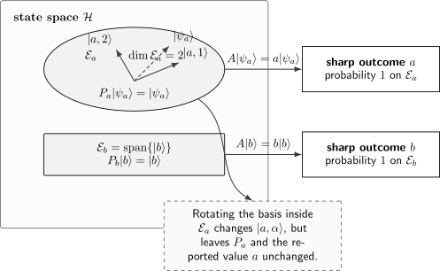
A sharp outcome labels an entire eigenspace. Within the degenerate space $\mathcal E_a$, the orthonormal basis vectors $|a,1\rangle$ and $|a,2\rangle$ are not unique; the projector $P_a$ and the outcome $a$ are.

Eigenstates as Definite-Value States

Let $A$ be a self-adjoint observable with a discrete eigenvalue $a$, and let $P_a$ be the orthogonal projector onto $\mathcal E_a$. For a normalized pure state, the following statements are equivalent:

$$\begin{aligned} A|\psi\rangle&=a|\psi\rangle,\\ |\psi\rangle&\in\mathcal E_a,\\ P_a|\psi\rangle&=|\psi\rangle,\\ \langle\psi|P_a|\psi\rangle&=1. \end{aligned}$$

The last line is the Born-rule statement that outcome $a$ occurs with certainty. To see why probability one implies membership in the eigenspace, note that

$$\begin{aligned} \|(I-P_a)|\psi\rangle\|^2 &=\langle\psi|(I-P_a)|\psi\rangle\\ &=1-\langle\psi|P_a|\psi\rangle\\ &=0. \end{aligned}$$

Therefore $(I-P_a)|\psi\rangle=0$ and $P_a|\psi\rangle=|\psi\rangle$.

Certainty is observable-relative

The phrase “the system is in an eigenstate” is incomplete unless the operator is named. A state can be an eigenstate of $A$ and a superposition of eigenstates of $B$. For a spin-one-half system, $|{+z}\rangle$ is an eigenstate of $S_z$ but

$$|{+z}\rangle = \frac{|{+x}\rangle+|{-x}\rangle}{\sqrt2},$$

so an $S_x$ measurement has two possible outcomes.

Every state is an eigenstate of the identity:

$$I|\psi\rangle=|\psi\rangle.$$

Being an eigenstate is therefore not an intrinsic measure of how “classical” or “simple” a state is. It records definiteness relative to a chosen operator.

Self-Adjoint Operators and Orthogonality

Reality of eigenvalues

Let $A=A^\dagger$ and let $|a\rangle$ be a nonzero eigenvector in its domain. The eigenvalue equation gives

$$\langle a|A|a\rangle = a\langle a|a\rangle.$$

The expectation on the left is real:

$$\begin{aligned} \langle a|A|a\rangle^* &=\langle a|A^\dagger|a\rangle\\ &=\langle a|A|a\rangle. \end{aligned}$$

Because $\langle a|a\rangle>0$ is real, the eigenvalue $a$ must be real. This argument concerns normalizable eigenvectors; the full statement that the spectrum of a self-adjoint operator is real is stronger and belongs to the spectral theorem.

Orthogonality of distinct eigenspaces

Eigenvectors of a self-adjoint operator belonging to distinct eigenvalues are orthogonal. Suppose

$$A|a\rangle=a|a\rangle, \qquad A|b\rangle=b|b\rangle, \qquad a\ne b.$$

Self-adjointness gives

$$\begin{aligned} b\langle a|b\rangle &=\langle a|Ab\rangle\\ &=\langle Aa|b\rangle\\ &=a\langle a|b\rangle, \end{aligned}$$

Hence

$$(a-b)\langle a|b\rangle=0,$$

and $a\ne b$ implies

$$\langle a|b\rangle=0.$$

Within a degenerate eigenspace, arbitrary eigenvectors need not initially be orthogonal, but one can choose an orthonormal basis by Gram–Schmidt orthogonalization. The basis choice is conventional; the eigenspace is not.

This conclusion depends on the operator class. A nonnormal matrix can have eigenvectors for distinct eigenvalues that are not orthogonal. Orthogonality is not a generic consequence of the eigenvalue equation alone.

Degeneracy

An eigenvalue $a$ is degenerate when its eigenspace contains more than one independent direction. Choose an orthonormal basis

$$\left\{ |a,\alpha\rangle \right\}_{\alpha=1}^{g_a}$$

for that eigenspace. The spectral projector is

$$P_a = \sum_{\alpha=1}^{g_a} |a,\alpha\rangle\langle a,\alpha|.$$

Although the individual basis vectors can be changed by a unitary rotation inside $\mathcal E_a$, the projector is unchanged. If

$$|a,\mu\rangle' = \sum_\alpha U_{\mu\alpha}|a,\alpha\rangle,$$

with $U$ unitary on the eigenspace, then

$$\sum_\mu |a,\mu\rangle'\langle a,\mu|' = P_a.$$

The observable therefore identifies the subspace, not a privileged basis inside it.

Measurement does not resolve a degeneracy by itself

An ideal measurement of $A$ reports the value $a$. It does not determine the degeneracy label $\alpha$ unless the apparatus measures additional information. For a state

$$|\psi\rangle = \sum_{a,\alpha} c_{a\alpha}|a,\alpha\rangle,$$

the probability of outcome $a$ is

$$p(a) = \langle\psi|P_a|\psi\rangle = \sum_\alpha|c_{a\alpha}|^2.$$

The separate numbers $|c_{a\alpha}|^2$ are not probabilities for outcomes of $A$ alone, because $\alpha$ is not among that observable’s reported values.

State update in a degenerate eigenspace

In the Lüders update model, observing $a$ gives

$$|\psi\rangle \longmapsto \frac{P_a|\psi\rangle} {\sqrt{\langle\psi|P_a|\psi\rangle}}.$$

This preserves coherence among components inside $\mathcal E_a$. The PVM for $A$ determines the outcome probabilities, but it does not uniquely determine every possible physical instrument. A more detailed apparatus can disturb, rotate, or resolve states within the degenerate subspace while reporting the same coarse outcome. See Degenerate Measurements and Lüders Rule for the canonical update discussion.

Complete Sets of Eigenstates

For a self-adjoint operator on a finite-dimensional Hilbert space, the spectral theorem guarantees an orthonormal basis of eigenvectors. If $a$ runs over distinct eigenvalues and $\alpha$ over a basis within each eigenspace, then

$$I = \sum_a P_a = \sum_{a,\alpha} |a,\alpha\rangle\langle a,\alpha|.$$

Every vector can therefore be expanded as

$$|\psi\rangle = \sum_{a,\alpha} c_{a\alpha}|a,\alpha\rangle, \qquad c_{a\alpha} = \langle a,\alpha|\psi\rangle.$$

For a normalized state,

$$\sum_{a,\alpha}|c_{a\alpha}|^2=1.$$

The expansion coefficients are state-dependent amplitudes. They are not eigenvalues. The eigenvalues are properties of $A$; the coefficients describe the chosen state relative to an eigenbasis of $A$.

Projector form is basis-independent

Grouping degenerate components gives

$$|\psi\rangle = \sum_a P_a|\psi\rangle.$$

This form does not choose a basis inside any eigenspace. It is often the cleanest statement of completeness when degeneracy matters.

Completeness is not automatic for every operator

A generic finite-dimensional matrix can fail to possess enough independent eigenvectors to span the space. A nonnormal operator can be diagonalizable without having an orthonormal eigenbasis. Self-adjoint operators avoid both problems in finite dimension.

In infinite dimension, completeness may involve countable sums, continuous spectral integrals, or both. One should not write

$$I=\sum_n|a_n\rangle\langle a_n|$$

unless the stated eigenvectors really form a complete orthonormal basis for the space under discussion.

Spectral Decomposition

With the same finite-dimensional assumptions, a self-adjoint operator can be reconstructed from its distinct eigenvalues and eigenspace projectors:

$$A=\sum_a aP_a.$$

Acting on a vector in $\mathcal E_b$ gives

$$A|\psi_b\rangle = \sum_a aP_a|\psi_b\rangle = b|\psi_b\rangle.$$

This decomposition explains why the physically invariant object associated with a degenerate outcome is $P_a$, not a chosen list of basis vectors. Derivations and operator-function applications belong to Spectral Decomposition.

If $f$ is defined on the spectrum, then

$$f(A)|a,\alpha\rangle = f(a)|a,\alpha\rangle.$$

Different eigenvalues of $A$ can become the same eigenvalue of $f(A)$. Thus an operator function can increase degeneracy. For example, $S_z$ distinguishes $m$ from $-m$, whereas $S_z^2$ does not.

Measurement Outcomes

For a purely discrete sharp observable,

$$A=\sum_a aP_a,$$

the Born rule assigns

$$p(a|\psi) = \langle\psi|P_a|\psi\rangle.$$

If the state is an $a$ eigenstate, then $P_a|\psi\rangle=|\psi\rangle$ and

$$p(a|\psi)=1, \qquad p(b|\psi)=0 \quad \text{for }b\ne a.$$

Conversely, a generic superposition across distinct eigenspaces produces a probability distribution over eigenvalues. The detailed calculation workflow is Born Rule for Discrete Spectra.

Outcome, eigenvalue, and expectation value

These three quantities should be kept distinct:

• An eigenvalue is a possible sharp outcome encoded by the observable.
• An outcome is the value recorded in one run.
• An expectation value is the probability-weighted ensemble mean.

For

$$|\psi\rangle = \sum_{a,\alpha} c_{a\alpha}|a,\alpha\rangle,$$

the expectation is

$$\langle A\rangle_\psi = \sum_a a\,p(a|\psi).$$

It need not equal any eigenvalue. For $\sigma_z$ in the state $(|0\rangle+|1\rangle)/\sqrt2$, the possible outcomes are $\pm1$, while the expectation value is zero.

Probability one is not a claim about hidden preexisting values

Within the operational formalism, an eigenstate predicts a definite result for the corresponding ideal sharp measurement. This statement alone does not settle whether unmeasured observables possessed context-independent values before measurement. That interpretive question requires additional assumptions and belongs to the foundations volumes.

Zero Variance Characterization

For a normalized state in the domain of a self-adjoint $A$, define

$$\mu=\langle\psi|A|\psi\rangle.$$

The variance can be written as

$$(\Delta A)^2_\psi = \|(A-\mu I)|\psi\rangle\|^2,$$

under the usual domain assumptions. Therefore,

$$\Delta A=0 \quad\Longleftrightarrow\quad (A-\mu I)|\psi\rangle=0.$$

Equivalently,

$$\Delta A=0 \quad\Longleftrightarrow\quad A|\psi\rangle=\mu|\psi\rangle.$$

Thus a normalized pure state has zero spread in a sharp observable exactly when it is an eigenstate of that observable. This is stronger than merely having a known expectation value.

For unbounded operators, the norm expression requires $|\psi\rangle$ to be in the appropriate domain. Writing $\langle A^2\rangle-\langle A\rangle^2$ additionally requires the second moment to exist.

Example: Spin One-Half

The $z$ component of spin is

$$S_z = \frac{\hbar}{2}\sigma_z = \frac{\hbar}{2} \begin{pmatrix} 1&0\\ 0&-1 \end{pmatrix}.$$

Its normalized eigenstates satisfy

$$\begin{aligned} S_z|{+z}\rangle &=\frac{\hbar}{2}|{+z}\rangle,\\ S_z|{-z}\rangle &=-\frac{\hbar}{2}|{-z}\rangle. \end{aligned}$$

A general normalized spin state can be written

$$|\psi\rangle = \cos\frac{\theta}{2}|{+z}\rangle +e^{i\phi}\sin\frac{\theta}{2}|{-z}\rangle.$$

An ideal $S_z$ measurement gives

$$\begin{aligned} \Pr\left(+\frac{\hbar}{2}\right) &=\cos^2\frac{\theta}{2},\\ \Pr\left(-\frac{\hbar}{2}\right) &=\sin^2\frac{\theta}{2}. \end{aligned}$$

Only at the poles, $\theta=0$ or $\theta=\pi$, is the state an $S_z$ eigenstate. The relative phase $\phi$ does not affect these two probabilities, but it matters for spin components in other directions.

Example: Degenerate Spin Observable

For spin one,

$$S_z|m\rangle=\hbar m|m\rangle, \qquad m\in\{-1,0,1\}.$$

The squared operator has action

$$S_z^2|m\rangle = \hbar^2m^2|m\rangle.$$

Its two distinct eigenvalues and projectors are

$$\begin{aligned} P_{\hbar^2} &=|1\rangle\langle1| +|-1\rangle\langle-1|,\\ P_0 &=|0\rangle\langle0|. \end{aligned}$$

The eigenvalue $\hbar^2$ is twofold degenerate. Every normalized state

$$|\psi\rangle = \alpha|1\rangle+\beta|-1\rangle, \qquad |\alpha|^2+|\beta|^2=1,$$

is an eigenstate of $S_z^2$ with eigenvalue $\hbar^2$, although it need not be an eigenstate of $S_z$. A measurement of $S_z^2$ alone cannot distinguish the sign of $m$.

Example: Diagonalizing a Two-Level Observable

Consider

$$A= \begin{pmatrix} 3&1\\ 1&3 \end{pmatrix}.$$

The characteristic equation is

$$\det(A-aI) = (3-a)^2-1 = 0,$$

so the eigenvalues are $a_+=4$ and $a_-=2$. Normalized eigenvectors are

$$|a_+\rangle = \frac{1}{\sqrt2} \begin{pmatrix} 1\\ 1 \end{pmatrix}, \qquad |a_-\rangle = \frac{1}{\sqrt2} \begin{pmatrix} 1\\ -1 \end{pmatrix}.$$

They are orthogonal, and

$$A = 4|a_+\rangle\langle a_+| +2|a_-\rangle\langle a_-|.$$

The standard basis vectors are not eigenvectors of $A$. For example,

$$\begin{pmatrix} 1\\ 0 \end{pmatrix} = \frac{|a_+\rangle+|a_-\rangle}{\sqrt2},$$

so an $A$ measurement in that state yields $4$ or $2$, each with probability $1/2$.

The general matrix algorithm and distinctions between algebraic and geometric multiplicity are developed in Eigenvalues and Eigenvectors and Diagonalization.

Example: Energy Eigenstates

For a Hamiltonian with discrete eigenstates,

$$H|E_n,\alpha\rangle = E_n|E_n,\alpha\rangle.$$

These are eigenstates of the energy observable. If the Hamiltonian is time-independent, unitary evolution gives

$$e^{-iHt/\hbar}|E_n,\alpha\rangle = e^{-iE_nt/\hbar}|E_n,\alpha\rangle.$$

Only a global phase changes, so the physical ray is stationary. A superposition of different energies acquires relative phases and generally changes as a ray. The dynamics and continuum caveats are developed in Energy Eigenstates.

Degenerate energy eigenstates can evolve with the same common phase under the unperturbed Hamiltonian. Additional commuting observables or perturbations may distinguish states inside the degenerate energy subspace.

Commuting Observables and Shared Eigenstates

If two finite-dimensional self-adjoint operators commute,

$$[A,B]=0,$$

then each eigenspace of $A$ is invariant under $B$. Indeed, for $|\psi\rangle\in\mathcal E_a$,

$$A(B|\psi\rangle) = B(A|\psi\rangle) = aB|\psi\rangle.$$

Thus $B|\psi\rangle$ remains in $\mathcal E_a$. Diagonalizing $B$ within every degenerate eigenspace of $A$ produces a common orthonormal eigenbasis.

Two cautions matter:

1. If $A$ is degenerate, an arbitrary $A$ eigenvector need not already be a $B$ eigenvector.
2. A common eigenvector does not by itself imply that $A$ and $B$ commute on the whole space.

A collection of commuting observables can refine degenerate labels until their joint eigenvalues identify rays. That is the purpose of a Complete Set of Commuting Observables.

Mixed States with a Definite Value

The word eigenstate usually refers to a pure state ray, but definiteness of an observable also makes sense for density operators. A density operator $\rho$ has definite value $a$ when its support lies entirely in $\mathcal E_a$:

$$P_a\rho P_a=\rho.$$

Equivalently,

$$\operatorname{Tr}(\rho P_a)=1.$$

If $a$ is nondegenerate, the only such density operator is the pure projector

$$\rho=|a\rangle\langle a|.$$

If $a$ is degenerate, mixtures and coherent pure states supported in $\mathcal E_a$ all have the same definite value. For example,

$$\rho = \frac12|a,1\rangle\langle a,1| +\frac12|a,2\rangle\langle a,2|$$

is mixed but yields $a$ with certainty. Definite value therefore does not imply purity when degeneracy is present.

Continuous-Spectrum Caveat

The equation

$$\hat x|x\rangle=x|x\rangle$$

is useful notation, but $|x\rangle$ is not a normalizable vector in $L^2(\mathbb R)$. Likewise, plane-wave momentum states do not belong to the ordinary Hilbert space. They are generalized eigenvectors normalized with Dirac deltas rather than Kronecker deltas.

A self-adjoint operator may have spectral values that are not Hilbert-space eigenvalues. Exact position on the line is the standard example: every real number lies in the spectrum of $\hat x$, but there is no normalizable state with probability one at a single point.

The precise replacement for a sum of eigenprojectors is a projection-valued measure:

$$A = \int_{\mathbb R} \lambda\,dP(\lambda).$$

Finite-resolution statements use projectors $P(\Delta)$ for intervals $\Delta$, not rank-one projectors onto normalizable exact-position states. See Generalized Eigenvectors for the mathematical bridge.

Infinite-Dimensional and Domain Caveats

For an unbounded operator, an eigenvector must belong to $\mathcal D(A)$. A formal solution of a differential equation is not automatically an eigenvector: it must satisfy square-integrability, regularity, boundary conditions, and any other domain requirements.

For example, solving

$$-i\hbar\frac{d\psi}{dx}=p\psi$$

on the real line gives a plane wave, but the plane wave is not in $L^2(\mathbb R)$. It represents a generalized momentum eigenstate, not a normalizable vector in the Hilbert space.

On a circle or finite interval with suitable boundary conditions, related differential expressions can instead possess normalizable discrete eigenvectors. The domain and configuration space determine which conclusion is correct.

A Practical Eigenstate Audit

When a calculation claims that a state is an eigenstate, check:

1. Operator: Which observable or operator is being named?
2. Space and domain: Does the proposed vector belong to the Hilbert space and to $\mathcal D(A)$?
3. Nonzero vector: Has the zero solution been excluded?
4. Equation: Does applying $A$ return one scalar multiple of the original vector?
5. Units: Does the proposed eigenvalue carry the operator’s dimensions?
6. Normalization: Is a normalized representative needed for the physical probability statement?
7. Degeneracy: Is the outcome associated with a ray or an entire eigenspace?
8. Projector: What is the basis-independent $P_a$?
9. Completeness: Do the stated eigenvectors actually span the relevant space?
10. Spectrum type: Is the proposed state normalizable, or is it a generalized continuous-spectrum vector?
11. Measurement model: Does probability one concern only the outcome, or has a post-measurement update also been specified?

Common Mistakes

• Assuming every state is an eigenstate of the observable being measured. A generic state is a superposition across several eigenspaces.
• Allowing the zero vector as an eigenvector. It satisfies the equation for every scalar and carries no eigenvalue information.
• Confusing an eigenvalue with an expansion coefficient. Eigenvalues belong to the operator; amplitudes belong to the state in a chosen basis.
• Confusing an expectation value with an outcome. The ensemble mean need not lie in the spectrum.
• Treating one basis vector as the degenerate outcome. The invariant object is the entire eigenspace and its projector.
• Assuming an $A$ eigenstate is an eigenstate of every commuting $B$. This can fail inside a degenerate eigenspace until a common basis is chosen.
• Assuming any matrix has a complete orthonormal eigenbasis. This is guaranteed for finite-dimensional normal operators, including Hermitian matrices, not for arbitrary matrices.
• Calling every spectral value an eigenvalue. Continuous-spectrum points need not have normalizable eigenvectors.
• Treating exact position kets as ordinary unit vectors. They are distributional generalized eigenvectors.
• Assuming probability one uniquely fixes the preparation. A degenerate outcome can be certain for many pure and mixed states.
• Inferring a unique state-update rule from the eigenvalue equation. Outcome statistics and measurement disturbance are separate structures.
• Ignoring boundary conditions in differential eigenvalue problems. They are part of the operator and determine the allowed spectrum.

Interpretation Boundary

Eigenstates provide the formal language of definite outcomes for sharp observables. They do not imply that every physical quantity has a simultaneous preexisting value. Nor do they say that an apparatus literally “reads the eigenvalue already stored in the wavefunction.” The formal statement is conditional and operational: given a state supported in $\mathcal E_a$, the specified ideal measurement returns $a$ with probability one.

For degenerate observables, this certainty does not identify a unique ray. For continuous observables, exact generalized eigenstates may be idealizations rather than preparable normalizable states. Precision comes from stating the operator, its spectral projector or measure, the state, and the measurement model.

Summary

• An eigenvector is a nonzero vector satisfying $A|a\rangle=a|a\rangle$.
• Nonzero scalar multiples represent the same eigenstate ray.
• The eigenspace is $\mathcal E_a=\ker(A-aI)$.
• A normalized eigenstate of a sharp observable yields its eigenvalue with probability one.
• Distinct eigenspaces of a self-adjoint operator are orthogonal.
• Degeneracy means one outcome corresponds to a multidimensional eigenspace; its projector is basis-independent.
• A finite-dimensional self-adjoint operator has a complete orthonormal eigenbasis and a spectral decomposition $A=\sum_a aP_a$.
• Zero variance is equivalent to being an eigenstate, under the appropriate domain assumptions.
• Mixed states can have a definite degenerate value when their support lies in one eigenspace.
• Continuous-spectrum generalized eigenvectors are not ordinary normalizable Hilbert-space states.

References

• P. A. M. Dirac, The Principles of Quantum Mechanics, 4th ed., Oxford University Press, 1958, Chapters I–III.
• J. von Neumann, Mathematical Foundations of Quantum Mechanics, Princeton University Press, 1955, Chapters II–III.
• R. Shankar, Principles of Quantum Mechanics, 2nd ed., Springer, 1994, Chapters 1 and 4.
• J. J. Sakurai and J. Napolitano, Modern Quantum Mechanics, 3rd ed., Cambridge University Press, 2020, Chapter 1.
• D. J. Griffiths and D. F. Schroeter, Introduction to Quantum Mechanics, 3rd ed., Cambridge University Press, 2018, Chapters 3–4.
• L. E. Ballentine, Quantum Mechanics: A Modern Development, World Scientific, 1998, Chapters 2–3.
• B. C. Hall, Quantum Theory for Mathematicians, Springer, 2013, Chapters 2–4.
• M. Reed and B. Simon, Methods of Modern Mathematical Physics, Volume I: Functional Analysis, revised and enlarged ed., Academic Press, 1980.

Exercises

Exercise 1: Scaling and the zero vector

Suppose $A|a\rangle=a|a\rangle$ with $|a\rangle\ne0$. Prove that every $c|a\rangle$ with $c\ne0$ is an eigenvector with the same eigenvalue. Explain why the proof does not make $|0\rangle$ an eigenvector.

Solution

Linearity gives

$$A(c|a\rangle) = cA|a\rangle = ca|a\rangle = a(c|a\rangle).$$

If $c\ne0$, then $c|a\rangle$ is nonzero and therefore is an eigenvector. Taking $c=0$ produces the zero vector, which satisfies

$$A|0\rangle=a|0\rangle$$

for every $a$. It cannot identify one eigenvalue or one direction, so it is excluded by definition.

Exercise 2: Spin probabilities and definiteness

For

$$|\psi\rangle = \frac{\sqrt3}{2}|{+z}\rangle +\frac{i}{2}|{-z}\rangle,$$

find the probabilities, expectation value, and variance for a measurement of $S_z$. Is the state an $S_z$ eigenstate?

Solution

The outcome probabilities are

$$\Pr\left(+\frac{\hbar}{2}\right)=\frac34, \qquad \Pr\left(-\frac{\hbar}{2}\right)=\frac14.$$

The expectation is

$$\langle S_z\rangle = \frac34\frac{\hbar}{2} +\frac14\left(-\frac{\hbar}{2}\right) = \frac{\hbar}{4}.$$

Since $S_z^2=(\hbar^2/4)I$,

$$\begin{aligned} (\Delta S_z)^2 &=\langle S_z^2\rangle-\langle S_z\rangle^2\\ &=\frac{\hbar^2}{4}-\frac{\hbar^2}{16}\\ &=\frac{3\hbar^2}{16}. \end{aligned}$$

The variance is nonzero and both outcomes have nonzero probability, so the state is not an $S_z$ eigenstate.

Exercise 3: Degeneracy of spin squared

For spin one, let

$$|\psi\rangle = \frac{|1\rangle+i|-1\rangle}{\sqrt2}.$$

Show that $|\psi\rangle$ is an eigenstate of $S_z^2$ but not of $S_z$. What does an $S_z^2$ measurement report with certainty?

Solution

Because both $|1\rangle$ and $|-1\rangle$ have squared magnetic quantum number one,

$$\begin{aligned} S_z^2|\psi\rangle &= \frac{\hbar^2|1\rangle+i\hbar^2|-1\rangle}{\sqrt2}\\ &=\hbar^2|\psi\rangle. \end{aligned}$$

Thus $|\psi\rangle$ is an $S_z^2$ eigenstate with eigenvalue $\hbar^2$. However,

$$S_z|\psi\rangle = \frac{\hbar|1\rangle-i\hbar|-1\rangle}{\sqrt2},$$

which is not one scalar multiple of $|\psi\rangle$. The $S_z^2$ measurement reports $\hbar^2$ with probability one and does not reveal the sign of $m$.

Exercise 4: Orthogonality theorem

Let $A=A^\dagger$ and let $|a\rangle$, $|b\rangle$ be eigenvectors with distinct eigenvalues. Prove that they are orthogonal. Which step would fail for a generic non-Hermitian operator?

Solution

Using the eigenvalue equations and self-adjointness,

$$\begin{aligned} a\langle a|b\rangle &=\langle Aa|b\rangle\\ &=\langle a|A^\dagger b\rangle\\ &=\langle a|Ab\rangle\\ &=b\langle a|b\rangle. \end{aligned}$$

Therefore

$$(a-b)\langle a|b\rangle=0.$$

Since $a\ne b$, it follows that $\langle a|b\rangle=0$. For a generic non-Hermitian operator, replacing the action on the bra side by the same operator acting on the ket side is not justified; $A^\dagger\ne A$.

Exercise 5: Zero variance implies an eigenstate

For normalized $|\psi\rangle$ and self-adjoint $A$, assume all required domain conditions. Let $\mu=\langle A\rangle_\psi$. Starting from

$$(\Delta A)^2 = \|(A-\mu I)|\psi\rangle\|^2,$$

prove that $\Delta A=0$ if and only if $|\psi\rangle$ is an eigenstate of $A$.

Solution

A norm is zero exactly when its vector is zero. Hence

$$\Delta A=0 \quad\Longleftrightarrow\quad (A-\mu I)|\psi\rangle=0.$$

Rearranging gives

$$A|\psi\rangle=\mu|\psi\rangle.$$

Thus the state is an eigenstate with eigenvalue $\mu$. Conversely, if $A|\psi\rangle=a|\psi\rangle$, then $\mu=a$ and $(A-\mu I)|\psi\rangle=0$, so the variance vanishes.

Exercise 6: Diagonalize a two-level operator

Find the normalized eigenvectors of

$$A= \begin{pmatrix} 2&i\\ -i&2 \end{pmatrix},$$

and write its spectral decomposition.

Solution

The characteristic polynomial is

$$\det(A-aI) = (2-a)^2-1,$$

so $a_+=3$ and $a_-=1$. One normalized choice is

$$|a_+\rangle = \frac{1}{\sqrt2} \begin{pmatrix} i\\ 1 \end{pmatrix}, \qquad |a_-\rangle = \frac{1}{\sqrt2} \begin{pmatrix} -i\\ 1 \end{pmatrix}.$$

Direct substitution verifies the eigenvalue equations, and the two vectors are orthogonal. Therefore

$$A = 3|a_+\rangle\langle a_+| +|a_-\rangle\langle a_-|.$$

Exercise 7: Commutation and a degenerate eigenspace

On $\mathbb C^3$, let

$$A= \begin{pmatrix} 1&0&0\\ 0&1&0\\ 0&0&2 \end{pmatrix}, \qquad B= \begin{pmatrix} 1&0&0\\ 0&-1&0\\ 0&0&0 \end{pmatrix}.$$

Verify that $[A,B]=0$. Give an eigenvector of $A$ that is not an eigenvector of $B$, and then give a common eigenbasis.

Solution

Both matrices are diagonal, so $AB=BA$ and their commutator vanishes. The eigenvalue-one eigenspace of $A$ is the span of the first two standard basis vectors. The vector

$$|\psi\rangle = \frac{1}{\sqrt2} \begin{pmatrix} 1\\ 1\\ 0 \end{pmatrix}$$

is an $A$ eigenvector with eigenvalue one, but

$$B|\psi\rangle = \frac{1}{\sqrt2} \begin{pmatrix} 1\\ -1\\ 0 \end{pmatrix}$$

is not proportional to $|\psi\rangle$. The standard basis vectors form a common eigenbasis. This shows why commutation guarantees that a common basis can be chosen, not that every vector in a degenerate eigenspace is already a joint eigenvector.

Exercise 8: A mixed state with definite value

Let $P_a$ project onto a two-dimensional eigenspace spanned by $|a,1\rangle$ and $|a,2\rangle$, and define

$$\rho = q|a,1\rangle\langle a,1| +(1-q)|a,2\rangle\langle a,2|, \qquad 0<q<1.$$

Show that outcome $a$ has probability one. Is $\rho$ pure?

Solution

Because both basis vectors lie in the range of $P_a$,

$$P_a\rho P_a=\rho.$$

The outcome probability is

$$\operatorname{Tr}(\rho P_a) = \operatorname{Tr}\rho = 1.$$

For $0<q<1$,

$$\operatorname{Tr}(\rho^2) = q^2+(1-q)^2 <1,$$

so $\rho$ is mixed. A degenerate observable can therefore have a definite value in a mixed state.

Exercise 9: Normalizable or generalized?

Solve the formal momentum eigenvalue equation on the real line,

$$-i\hbar\frac{d\psi_p}{dx} = p\psi_p.$$

Explain why its nonzero solutions are not ordinary eigenvectors in $L^2(\mathbb R)$.

Solution

The differential equation gives

$$\psi_p(x)=Ce^{ipx/\hbar}.$$

Its modulus is constant:

$$|\psi_p(x)|^2=|C|^2.$$

For $C\ne0$,

$$\int_{-\infty}^{\infty} |\psi_p(x)|^2\,dx = \infty.$$

The plane wave is therefore not in $L^2(\mathbb R)$ and is not a normalizable Hilbert-space eigenvector. It is a generalized eigenfunction, interpreted distributionally and used inside momentum-space expansions.