Observables

An observable is a physical quantity whose possible measurement outcomes and outcome probabilities are encoded by an operator-valued measurement rule. For a standard sharp real-valued observable, that rule is represented by a self-adjoint operator or, equivalently, its projection-valued spectral measure. More general observables are represented by positive-operator-valued measures.

This definition is deliberately broader than the classroom slogan “observables are Hermitian matrices.” Hermitian matrices are the correct finite-dimensional representatives of sharp observables, but they do not by themselves describe every realistic measurement, continuous outcome space, or post-measurement state change.

The term observable is used in two closely related ways:

• for the physical quantity or experimental question, such as energy, a spin component, or whether a detector clicks;
• for the mathematical outcome rule assigned to that question, such as a self-adjoint operator, PVM, or POVM.

The intended meaning should be clear from context. This page keeps the physical and mathematical layers visible rather than collapsing them into one symbol.

The Observable Is a Question About Outcomes

A classical observable is often a function on phase space. If the classical state is known, the function has one definite value. A quantum observable has a different role: together with a quantum state, it determines a probability distribution over possible records.

The basic ingredients are:

1. an outcome space $\Omega$;
2. a rule assigning an operator to each allowed outcome event;
3. a prepared state $\rho$;
4. the probability law obtained from state and observable together.

For an event $X\subseteq\Omega$, write the assigned effect as $E(X)$. Then

$$p_\rho(X) = \operatorname{Tr} \left[ \rho E(X) \right].$$

The state alone does not determine this distribution. The observable alone does not either. A probability law emerges from their pairing.

Five Objects, Five Roles

The following distinctions organize the rest of the page.

Object	Role	Typical notation
Physical quantity	identifies what is being asked	energy, position, $S_z$
Observable	assigns effects to outcome events	$E(X)$ or self-adjoint $A$
State	describes the preparation	$\rho$ or $\lvert\psi\rangle$
Outcome law	predicts record frequencies	$p_\rho(X)$
Instrument or apparatus	implements records and disturbances	$\mathcal I_X$ plus a device model

These objects are related, but none should be substituted blindly for another. In particular, an observable specifies probabilities; it does not usually specify a unique physical apparatus or state-update mechanism.

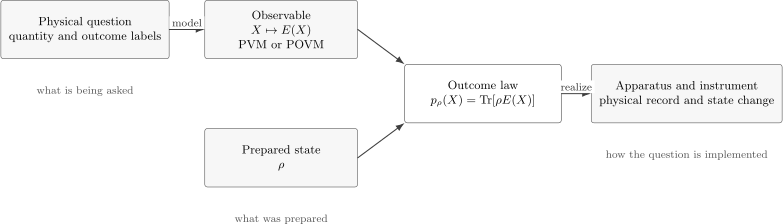
An observable and a state determine outcome probabilities. An apparatus and instrument add the physical implementation, record production, and conditional state change. Applying an operator to a ket is not this whole chain.

Sharp Real-Valued Observables

A standard sharp real-valued observable is represented by a self-adjoint operator $A$. In finite dimension, this is a Hermitian matrix:

$$A^\dagger=A.$$

Its spectral decomposition is

$$A = \sum_a aP_a,$$

where the sum runs over distinct eigenvalues and $P_a$ projects onto the full eigenspace associated with $a$. The projectors satisfy

$$P_aP_b = \delta_{ab}P_a, \qquad \sum_a P_a=I.$$

The eigenvalues are the possible numerical outcomes. The projectors determine their probabilities. Both pieces matter.

Why Self-Adjointness Matters

For a sharp real-valued observable, self-adjointness provides the spectral structure needed for a real probability distribution:

• spectral values are real;
• disjoint spectral events correspond to orthogonal projectors;
• the spectral projectors resolve the identity;
• functions of the outcome value correspond to functions of the operator.

In finite dimension, Hermitian and self-adjoint mean the same thing. For unbounded operators such as position and momentum, the domain and boundary conditions are part of the operator. A formally Hermitian differential expression is not automatically a self-adjoint observable. The precise warning belongs to Hermitian vs Self-Adjoint Operators.

The Spectral Measure Is the Full Sharp Observable

The discrete formula can hide the more general structure. A self-adjoint operator $A$ has a projection-valued measure, or PVM,

$$X \longmapsto P_A(X),$$

where $X$ is a measurable subset of the real outcome line. The operator is recovered as a spectral integral:

$$A = \int_{\mathbb R} a\,dP_A(a).$$

For a discrete spectrum,

$$P_A(X) = \sum_{a\in X}P_a.$$

For a continuous spectrum, $P_A(X)$ projects onto the subspace whose spectral values lie in the set $X$. This event-based language avoids pretending that every continuous outcome has a normalizable eigenket.

Probability Distribution of a Sharp Observable

Given a density operator $\rho$, the probability that a sharp measurement of $A$ yields a value in $X$ is

$$\Pr_\rho(A\in X) = \operatorname{Tr} \left[ \rho P_A(X) \right].$$

For a discrete pure-state measurement,

$$p_\psi(a) = \langle\psi\vert P_a\vert\psi\rangle.$$

For a mixed state,

$$p_\rho(a) = \operatorname{Tr}(\rho P_a).$$

These are instances of the Born Rule. This page uses the rule to characterize observables; the Born-rule page owns its systematic probability treatment.

Probability Density Is Not Probability

For a continuous observable, a point generally has probability zero. If the observable admits a density $p_\rho(a)$ relative to $da$, then

$$\Pr_\rho(A\in X) = \int_X da\,p_\rho(a).$$

The density can exceed one and carries inverse units of the outcome variable. Only its integral over a measurable region is a probability.

Not every spectral distribution needs to be expressed by a density. The PVM formula

$$\Pr_\rho(A\in X) = \operatorname{Tr} \left[ \rho P_A(X) \right]$$

remains valid for discrete, continuous, and mixed spectral types.

Definite Values and Eigenstates

A normalized state has a sharp value $a$ for the observable $A$ when

$$P_a\lvert\psi\rangle = \lvert\psi\rangle.$$

Equivalently in the discrete case,

$$A\lvert\psi\rangle = a\lvert\psi\rangle.$$

Then

$$p_\psi(a)=1.$$

Most states are not eigenstates of a given observable. For those states, the formalism supplies a distribution of possible outcomes, not one hidden eigenvalue selected merely by ignorance. The detailed language of eigenspaces and degeneracy belongs to Eigenvalues and Eigenstates.

Degenerate Outcomes

An outcome value may correspond to a subspace rather than one ray. If

$$A = \sum_a aP_a$$

and $\operatorname{rank}P_a>1$, then the outcome $a$ is degenerate. Learning $a$ tells us only that the state is associated with the subspace $\operatorname{ran}P_a$ in the ideal sharp model.

The observable does not distinguish vectors within that eigenspace. A more refined measurement may measure additional compatible quantities and split the degeneracy. Treating every $P_a$ as rank one secretly changes the observable.

Outcome Labels Versus Eigenvectors

The numerical value $a$ labels an outcome. The projector $P_a$ represents the event that this outcome occurs. Individual basis vectors inside $\operatorname{ran}P_a$ are not separate outcomes unless the measurement is refined to distinguish them.

This is why the canonical spectral sum runs over distinct values:

$$A = \sum_{a\in\operatorname{spec}(A)}aP_a,$$

not over an arbitrarily chosen eigenbasis with repeated copies of the same outcome label.

Expectation Value

The expectation value is the mean of the observable’s outcome distribution. For a discrete sharp observable,

$$\begin{aligned} \mathbb E_\rho[A] &= \sum_a a\,p_\rho(a) \\ &= \operatorname{Tr}(\rho A). \end{aligned}$$

For a normalized pure state,

$$\langle A\rangle_\psi = \langle\psi\vert A\vert\psi\rangle.$$

The expectation value is generally not an allowed outcome. If a qubit observable has outcomes $\pm1$ with equal probability, its expectation is $0$, even though $0$ is never observed in one trial.

The full statistical interpretation belongs to Expectation Values.

Variance and Higher Moments

The variance of a sharp observable is

$$(\Delta A)^2_\rho = \operatorname{Tr} \left[ \rho \left(A-\langle A\rangle_\rho I\right)^2 \right].$$

Equivalently,

$$(\Delta A)^2_\rho = \langle A^2\rangle_\rho - \langle A\rangle_\rho^2.$$

For a normalized pure state in the domain of the required products,

$$\Delta A=0$$

exactly when the state lies in an eigenspace of $A$. Domain assumptions matter for unbounded observables: a normalizable state can fail to have a finite second moment. See Variance and Standard Deviation.

Functions and Relabellings of an Observable

If $f$ is a real function on the spectrum, then the observable $f(A)$ has the same spectral projectors with relabelled values:

$$f(A) = \sum_a f(a)P_a$$

in the discrete case, or

$$f(A) = \int_{\mathbb R} f(a)\,dP_A(a)$$

generally.

If $f$ is one-to-one on the spectrum, no outcome information is lost; only the labels change. If $f$ maps several spectral values to the same number, the new observable is a coarse graining. Its spectral projector for an output $y$ is

$$P_{f(A)}(y) = \sum_{a:f(a)=y}P_a.$$

The functional calculus itself belongs to Functions of Operators.

Units and Affine Calibration

An observable carries the units of its outcome labels. If an instrument is recalibrated by

$$b=\alpha a+\beta,$$

then the corresponding sharp operator is

$$B = \alpha A+\beta I.$$

The spectral projectors are unchanged when $\alpha\ne0$, while the numerical readout scale and origin change. Expectations transform as

$$\langle B\rangle = \alpha\langle A\rangle+\beta.$$

For $\alpha<0$, the ordering of outcome labels reverses. Calibration is part of connecting a dimensionless detector record to a physical quantity with units.

A Sharp Observable Is More Than Its Spectrum

Two observables can have the same list of eigenvalues and still ask different questions because their spectral projectors differ.

For a qubit,

$$\sigma_z = \begin{pmatrix} 1&0\\ 0&-1 \end{pmatrix}, \qquad \sigma_x = \begin{pmatrix} 0&1\\ 1&0 \end{pmatrix}$$

both have spectrum $\{+1,-1\}$. Yet they distinguish different pairs of rays and can assign different distributions to the same prepared state. The outcome set alone does not define the observable.

Same Observable, Different Basis Representation

An abstract observable does not depend on the coordinate basis used to display it. Under a passive unitary basis change with component rule $d=Sc$,

$$A_{\mathcal F} = S A_{\mathcal E}S^\dagger.$$

The state and every spectral projector transform consistently:

$$\rho_{\mathcal F} = S\rho_{\mathcal E}S^\dagger, \qquad (P_a)_{\mathcal F} = S(P_a)_{\mathcal E}S^\dagger.$$

Therefore

$$\operatorname{Tr} \left[ \rho_{\mathcal F}(P_a)_{\mathcal F} \right] = \operatorname{Tr} \left[ \rho_{\mathcal E}(P_a)_{\mathcal E} \right].$$

Changing coordinates is not changing the physical observable. Changing the spectral projectors implemented by an apparatus is. See Change of Basis.

Observable Versus Operator

An operator is a mathematical map. An observable is a physical quantity or outcome rule represented by suitable operators. Not every operator is an observable:

• unitary operators can represent time evolution or symmetry actions;
• lowering operators are generally not self-adjoint;
• Kraus operators describe state changes associated with measurement outcomes;
• projectors can represent yes/no events;
• self-adjoint operators represent standard sharp real-valued observables.

Conversely, a general POVM observable is represented by a family of positive operators rather than one self-adjoint operator on the system. The taxonomy of linear maps belongs to Operators.

Applying an Operator Is Not Measuring

The expression

$$A\lvert\psi\rangle$$

is an operator action. It produces another vector when $\lvert\psi\rangle\in\mathcal D(A)$. It is not by itself a measurement event, an outcome, a probability, or a normalized post-measurement state.

A sharp measurement of $A$ uses its spectral projectors to assign probabilities

$$p(a) = \langle\psi\vert P_a\vert\psi\rangle$$

and requires an additional update rule or instrument to describe what happens conditioned on the record. Confusing $A\lvert\psi\rangle$ with “the measured state” is a category error.

Observable Versus Apparatus

An observable is an abstract probability rule for outcomes. An apparatus is a physical system that couples to the target, amplifies or records information, and produces a readout.

Several apparatuses can realize the same observable statistics. For example, a spin component can be inferred through spatial separation, state-dependent fluorescence, or an ancilla-assisted protocol. If their calibrated effects are the same, they represent the same observable at the level of outcome probabilities even if their dynamics and disturbances differ.

Conversely, one apparatus can be configured to realize different observables by changing fields, pulse sequences, orientations, analysis software, or coarse-graining rules.

Observable Versus Instrument

A POVM or PVM gives probabilities. A quantum instrument gives both outcome probabilities and conditional state transformations. If $\mathcal I_X$ is the operation associated with records in $X$, then

$$p_\rho(X) = \operatorname{Tr} \left[ \mathcal I_X(\rho) \right].$$

The associated effect satisfies

$$\operatorname{Tr} \left[ \mathcal I_X(\rho) \right] = \operatorname{Tr} \left[ \rho E(X) \right]$$

for every state. Different instruments can have the same effects and therefore the same observable statistics while producing different post-measurement states.

The state-changing side belongs to Generalized Measurements Overview.

Generalized Observables and POVMs

A positive-operator-valued measure assigns an effect $E(X)$ to each measurable outcome event $X\subseteq\Omega$ such that:

$$E(X)\geq0, \qquad E(\Omega)=I,$$

and disjoint events add:

$$E \left( \bigcup_k X_k \right) = \sum_k E(X_k).$$

The probability law is

$$p_\rho(X) = \operatorname{Tr} \left[ \rho E(X) \right].$$

A PVM is the sharp special case in which every $E(X)$ is a projector and

$$E(X\cap Y) = E(X)E(Y).$$

General POVMs include noisy, inefficient, unsharp, overcomplete, and coarse-grained observables. The dedicated first treatment is POVMs: First Encounter.

Finite-Outcome POVMs

For outcomes $i=1,\ldots,n$, a POVM is a set of effects satisfying

$$E_i\geq0, \qquad \sum_{i=1}^{n}E_i=I.$$

The probabilities are

$$p_\rho(i) = \operatorname{Tr}(\rho E_i).$$

If

$$E_iE_j = \delta_{ij}E_i,$$

the effects are mutually orthogonal projectors and the measurement is projective. Otherwise the observable is generalized.

Why One Self-Adjoint First-Moment Operator Is Not Enough

Suppose a finite real-valued POVM has outcomes $x_i$. Its first-moment operator is

$$A_E = \sum_i x_iE_i.$$

Then

$$\mathbb E_\rho[x] = \operatorname{Tr}(\rho A_E).$$

However, different POVMs can have the same first-moment operator while having different higher moments and full distributions. The operator $A_E$ generally does not reconstruct the effects $E_i$.

For a sharp PVM, the self-adjoint operator and spectral measure determine each other through the spectral theorem. For a general POVM, calling the first moment “the observable operator” can discard essential statistical information.

Coarse Graining

Suppose a fine-grained observable has effects $E_i$, but the reported outcome $y$ groups several microscopic labels. If $g(i)=y$, the coarse-grained effects are

$$F_y = \sum_{i:g(i)=y}E_i.$$

They remain positive and complete:

$$F_y\geq0, \qquad \sum_y F_y=I.$$

Coarse graining loses information. Grouping outcomes of a sharp PVM produces higher-rank projectors and therefore remains sharp. More general stochastic readout noise can instead produce effects that are not projectors.

Noisy Readout as a Classical Post-Processing

Let a sharp observable have outcome probabilities $p(a)$, and suppose the detector reports $y$ with conditional probability $q(y\mid a)$. Then

$$p(y) = \sum_a q(y\mid a)p(a).$$

The effective POVM effects are

$$E_y = \sum_a q(y\mid a)P_a.$$

They satisfy

$$E_y\geq0, \qquad \sum_y E_y=I.$$

This separates quantum uncertainty in the underlying sharp distribution from classical detector noise in the readout channel. Real experiments can contain both.

Joint Observables and Compatibility

Two observables are jointly measurable when one measurement has a joint outcome space whose marginals reproduce the original observables. For sharp PVM observables, joint measurability is equivalent under standard conditions to commutation of their spectral projectors.

For bounded finite-dimensional sharp operators, a familiar criterion is

$$[A,B]=0.$$

Then a common refinement of spectral projectors gives a joint distribution. For general POVMs, compatibility is subtler: nonprojective observables can be jointly measurable even when no pair of sharp operators with the same labels would be.

The canonical sharp treatment belongs to Compatible Observables.

Noncommuting Observables

If sharp observables do not commute, they generally lack a common PVM that assigns simultaneous sharp values with the correct marginals. This is a structural statement about their measurement algebras, not merely an assertion that laboratory technology is imperfect.

Noncommutation can lead to:

• preparation uncertainty relations;
• order dependence in sequential measurements;
• measurement disturbance;
• absence of a common eigenbasis;
• complementarity of experimental arrangements.

These consequences are related but not identical. A commutator alone does not specify a detector model or conditional state update.

Position

For a particle on the line, the ideal sharp position observable is represented by the self-adjoint position operator $Q$ and its spectral measure $P_Q(X)$. For a wavefunction $\psi(x)$,

$$\Pr_\psi(Q\in X) = \int_X dx\,|\psi(x)|^2.$$

The formal expression

$$(Q\psi)(x)=x\psi(x)$$

is an operator representation. A real position detector has finite resolution, efficiency, acceptance, and noise, so its calibrated observable may be a smeared POVM rather than the ideal PVM.

Momentum

In the position representation,

$$(P\psi)(x) = -i\hbar\frac{d\psi}{dx}$$

on an appropriate domain. In momentum representation it acts by multiplication:

$$(P\phi)(p)=p\phi(p).$$

These are two representations of the same sharp observable when the operator, domain, and boundary conditions are fixed consistently. A time-of-flight or diffraction apparatus is a physical implementation whose inference model must be calibrated to the momentum observable it approximates.

Energy and the Hamiltonian

For a closed system with time-independent dynamics, the Hamiltonian $H$ is both the generator of time translation and the standard energy observable. Its spectral measure determines energy-outcome probabilities:

$$\Pr_\rho(H\in X) = \operatorname{Tr} \left[ \rho P_H(X) \right].$$

The dual role should not be conflated. Acting with $H$ in the Schrödinger equation generates evolution; measuring energy is a measurement procedure associated with the spectral data of $H$. The dynamical role belongs to Hamiltonians.

Spin Components

For spin $1/2$, the component along a unit direction $\boldsymbol n$ is

$$S_{\boldsymbol n} = \frac{\hbar}{2} \boldsymbol n\cdot\boldsymbol\sigma.$$

Its outcomes are

$$+\frac{\hbar}{2}, \qquad -\frac{\hbar}{2},$$

with projectors

$$P_\pm(\boldsymbol n) = \frac12 \left( I\pm \boldsymbol n\cdot\boldsymbol\sigma \right).$$

For a qubit state with Bloch vector $\boldsymbol r$,

$$p_\pm = \frac12 \left( 1\pm\boldsymbol r\cdot\boldsymbol n \right).$$

Changing $\boldsymbol n$ changes the physical observable, not merely its matrix representation in one fixed basis.

Local Observables on Composite Systems

For

$$\mathcal H_{AB} = \mathcal H_A\otimes\mathcal H_B,$$

an observable acting only on subsystem $A$ is represented as

$$A\otimes I_B.$$

Its expectation value is

$$\langle A\otimes I_B\rangle_\rho = \operatorname{Tr} \left[ \rho(A\otimes I_B) \right] = \operatorname{Tr}_A(\rho_A A),$$

where $\rho_A=\operatorname{Tr}_B\rho$. Local outcome statistics depend only on the reduced state, even when the global state is entangled. See Subsystems and Local Observables.

State Dependence and Observable Dependence

A probability distribution changes if either the state or the observable changes:

$$p_\rho(X) = \operatorname{Tr} \left[ \rho E(X) \right].$$

It is therefore useful to separate two questions:

1. Preparation question: which $\rho$ describes the ensemble?
2. Measurement question: which effects $E(X)$ describe the calibrated records?

Experiments that vary a control pulse before a fixed detector may be described as changing the state, changing the effective observable, or changing both, depending on where the unitary is placed in the model. The predicted probabilities agree when the descriptions are transformed consistently.

Heisenberg and Schrödinger Descriptions

Let $U(t)$ be unitary evolution. In the Schrödinger picture,

$$\rho(t) = U(t)\rho(0)U(t)^\dagger,$$

while a fixed observable has effects $E(X)$. In the Heisenberg picture, the state is fixed and the effects evolve:

$$E_t(X) = U(t)^\dagger E(X)U(t).$$

The outcome law is the same:

$$\operatorname{Tr} \left[ \rho(t)E(X) \right] = \operatorname{Tr} \left[ \rho(0)E_t(X) \right].$$

This equality reinforces the central point: physical predictions depend on the pairing of states and observables, not on which picture carries the time dependence.

Does an Observable Reveal a Pre-Existing Value?

The formalism predicts distributions and correlations for measurement outcomes. It does not generally license the classical inference that every observable had one context-independent eigenvalue before measurement.

An eigenstate gives a definite outcome for its associated sharp observable, but a generic state does not assign simultaneous sharp values to all observables. Noncommuting observables, contextuality results, and measurement disturbance make the classical hidden-value picture nontrivial and, under standard assumptions, untenable in general.

This page does not choose an interpretation of quantum mechanics. It records the minimal operational statement shared by the standard formalism: an observable and a state determine outcome probabilities.

What the Observable Formalism Does Not Settle

Specifying an observable does not by itself settle:

• how a particular apparatus couples to the system;
• which state update occurs after an outcome;
• whether the measurement is repeatable or nondemolition;
• how a macroscopic record becomes stable;
• whether the system possessed the outcome value before measurement;
• how to interpret individual outcomes;
• which approximations connect detector counts to an ideal target quantity.

Those questions require instruments, dynamics, decoherence, detector models, or interpretive assumptions. The boundary is treated explicitly in What the Measurement Formalism Does Not Settle.

An Observable Audit

Before trusting an observable calculation, record:

1. System Hilbert space: what degrees of freedom are modeled?
2. Outcome space: discrete labels, real values, bins, or detector records?
3. Observable type: self-adjoint operator/PVM or general POVM?
4. Units and calibration: what physical quantity do the labels represent?
5. State: pure, mixed, reduced, conditional, or time evolved?
6. Domain: is an unbounded operator defined on the relevant states?
7. Degeneracy: does one outcome correspond to a multidimensional subspace?
8. Distribution: do all probabilities remain nonnegative and normalized?
9. Update model: is a state change claimed, and if so, which instrument?
10. Implementation: what assumptions connect the apparatus to the abstract observable?

Common Mistakes

• Saying every observable is merely a Hermitian matrix without the finite-dimensional and sharp-observable qualifications.
• Treating an arbitrary operator as a measurable sharp observable.
• Applying $A$ to a ket and calling the result a measurement.
• Listing eigenvalues without the corresponding spectral projectors.
• Assuming the expectation value must be a possible outcome or the most likely outcome.
• Treating every state as an eigenstate of the measured observable.
• Replacing a degenerate spectral projector by arbitrarily chosen rank-one projectors.
• Using a probability density as though it were a dimensionless point probability.
• Assuming a POVM uniquely determines post-measurement states.
• Confusing a physical apparatus with the observable it is calibrated to realize.
• Ignoring domains and boundary conditions for unbounded observables.
• Inferring a common pre-existing value assignment for noncommuting observables from the notation alone.
• Describing detector noise as intrinsic quantum uncertainty without separating the readout model.

Further Connections

• Operators
• Eigenvalues and Eigenstates
• Discrete and Continuous Spectra
• Projectors
• Spectral Decomposition
• Born Rule
• Expectation Values
• Projective Measurement
• POVMs: First Encounter
• Generalized Measurements Overview

References

• P. A. M. Dirac, The Principles of Quantum Mechanics, 4th ed., Oxford University Press, 1958.
• J. von Neumann, Mathematical Foundations of Quantum Mechanics, Princeton University Press, 1955.
• R. Shankar, Principles of Quantum Mechanics, 2nd ed., Springer, 1994.
• J. J. Sakurai and J. Napolitano, Modern Quantum Mechanics, 3rd ed., Cambridge University Press, 2020.
• A. Peres, Quantum Theory: Concepts and Methods, Kluwer, 1995.
• K. Kraus, States, Effects, and Operations: Fundamental Notions of Quantum Theory, Springer, 1983.
• P. Busch, P. Lahti, J.-P. Pellonpää, and K. Ylinen, Quantum Measurement, Springer, 2016.
• E. B. Davies and J. T. Lewis, “An operational approach to quantum probability,” Communications in Mathematical Physics 17, 239–260, 1970.

Exercises

1. Same spectrum, different observable

Prepare the qubit state $\lvert0\rangle$. Compare the outcome distributions for $\sigma_z$ and $\sigma_x$. Why does their common spectrum not make them the same observable?

Solution

For $\sigma_z$, the spectral projectors are

$$P_+^{(z)} = \lvert0\rangle\langle0\rvert, \qquad P_-^{(z)} = \lvert1\rangle\langle1\rvert.$$

Therefore

$$p_z(+)=1, \qquad p_z(-)=0.$$

For $\sigma_x$, the projectors are

$$P_\pm^{(x)} = \lvert\pm\rangle\langle\pm\rvert,$$

where

$$\lvert\pm\rangle = \frac{ \lvert0\rangle\pm\lvert1\rangle }{\sqrt2}.$$

Thus

$$p_x(+)=p_x(-)=\frac12.$$

Both observables have outcomes $\pm1$, but their spectral projectors differ. The projectors determine which physical alternatives those labels denote.

2. Degenerate outcome

Let

$$A = 0 \left( \lvert0\rangle\langle0\rvert + \lvert1\rangle\langle1\rvert \right) + 2\lvert2\rangle\langle2\rvert.$$

For

$$\lvert\psi\rangle = \frac{ \lvert0\rangle+i\lvert1\rangle+\lvert2\rangle }{\sqrt3},$$

find the outcome probabilities. Does outcome $0$ identify a unique ray?

Solution

The spectral projectors are

$$P_0 = \lvert0\rangle\langle0\rvert + \lvert1\rangle\langle1\rvert, \qquad P_2 = \lvert2\rangle\langle2\rvert.$$

Therefore

$$p(0) = \langle\psi\vert P_0\vert\psi\rangle = \frac23,$$

and

$$p(2)=\frac13.$$

The outcome $0$ identifies the two-dimensional subspace $\operatorname{span}\{\lvert0\rangle,\lvert1\rangle\}$, not one ray. A more refined compatible observable would be needed to distinguish directions inside that subspace.

3. Expectation need not be an outcome

A sharp observable has outcomes $-2$ and $5$ with probabilities $3/4$ and $1/4$. Find its expectation and variance. Is the expectation an allowed outcome?

Solution

The expectation is

$$\langle A\rangle = \frac34(-2) + \frac14(5) = -\frac14.$$

The second moment is

$$\langle A^2\rangle = \frac34(4) + \frac14(25) = \frac{37}{4}.$$

Hence

$$\begin{aligned} (\Delta A)^2 &= \frac{37}{4} - \left(-\frac14\right)^2 \\ &= \frac{147}{16}. \end{aligned}$$

The expectation $-1/4$ is neither $-2$ nor $5$, so it is not a possible single-trial outcome.

4. Affine recalibration

Let a thermometer-like sharp observable $A$ have outcome values in degrees Celsius. A new readout reports

$$B=\frac95 A+32I.$$

How do its probabilities, expectation, and variance relate to those of $A$?

Solution

The new labels are

$$b=\frac95a+32.$$

Because this map is one-to-one, each event is carried to the corresponding event without changing its projector or probability. The expectation is

$$\langle B\rangle = \frac95\langle A\rangle+32.$$

Adding a constant does not change fluctuations, while multiplying by $9/5$ rescales them. Therefore

$$(\Delta B)^2 = \left(\frac95\right)^2 (\Delta A)^2.$$

5. A noisy binary readout

An ideal qubit measurement has projectors $P_+$ and $P_-$. The detector reports the wrong sign with probability $\epsilon$, where $0\leq\epsilon\leq1/2$. Find the two effective POVM effects.

Solution

The reported-plus effect is

$$E_+ = (1-\epsilon)P_+ + \epsilon P_-.$$

Similarly,

$$E_- = \epsilon P_+ + (1-\epsilon)P_-.$$

Both effects are positive, and

$$E_++E_- = P_++P_- = I.$$

When $\epsilon=0$, the POVM is the original PVM. When $\epsilon=1/2$, both effects equal $I/2$, so the reported sign is independent of the state.

6. Same first moment, different POVM

Consider three real outcome labels $-1,0,+1$. Compare the two POVMs

$$\begin{aligned} \mathsf E: &\quad E_{-1}=0, \quad E_0=I, \quad E_{+1}=0, \\ \mathsf F: &\quad F_{-1}=\frac12I, \quad F_0=0, \quad F_{+1}=\frac12I. \end{aligned}$$

Show that their first-moment operators agree but their distributions do not.

Solution

For $\mathsf E$,

$$A_{\mathsf E} = (-1)0+0I+(+1)0 = 0.$$

For $\mathsf F$,

$$A_{\mathsf F} = -\frac12I + \frac12I = 0.$$

Thus both have expectation zero in every state. But $\mathsf E$ reports $0$ with probability one, whereas $\mathsf F$ reports $-1$ and $+1$ with probability $1/2$ each. Their second moments also differ:

$$\mathbb E_{\mathsf E}[x^2]=0, \qquad \mathbb E_{\mathsf F}[x^2]=1.$$

The first-moment operator does not determine a general POVM.

7. Basis invariance of a sharp probability

Let $S$ be unitary, and define

$$\rho'=S\rho S^\dagger, \qquad P_a'=SP_aS^\dagger.$$

Show that the outcome probability is unchanged.

Solution

Using cyclicity of the trace and $S^\dagger S=I$,

$$\begin{aligned} \operatorname{Tr}(\rho'P_a') &= \operatorname{Tr} \left( S\rho S^\dagger SP_aS^\dagger \right) \\ &= \operatorname{Tr} \left( S\rho P_aS^\dagger \right) \\ &= \operatorname{Tr}(\rho P_a). \end{aligned}$$

The matrices changed, but the state-observable pairing and physical probability did not.

8. Observable versus instrument

Let a binary POVM have effects $E_0$ and $E_1$. Suppose one realization uses measurement operators $M_i$ with $M_i^\dagger M_i=E_i$. For outcome-dependent unitaries $U_i$, define $N_i=U_iM_i$. Show that the observable statistics are unchanged but the conditional states can differ.

Solution

The new effects are

$$N_i^\dagger N_i = M_i^\dagger U_i^\dagger U_iM_i = M_i^\dagger M_i = E_i.$$

Therefore both realizations assign

$$p(i) = \operatorname{Tr}(\rho E_i)$$

to each outcome. Their conditional output states are

$$\rho_i^{(M)} = \frac{M_i\rho M_i^\dagger}{p(i)}$$

and

$$\rho_i^{(N)} = U_i\rho_i^{(M)}U_i^\dagger.$$

These generally differ. The POVM fixes outcome statistics; the instrument also fixes state changes.