Operators

An operator is a map that acts on vectors, or more generally on other mathematical objects, in a quantum theory. For the state-vector formalism, the basic case is a linear map

$$A:\mathcal D(A)\longrightarrow\mathcal H,$$

where $\mathcal H$ is a Hilbert space and $\mathcal D(A)\subseteq\mathcal H$ is the operator’s domain. In finite-dimensional quantum mechanics one usually has $\mathcal D(A)=\mathcal H$. For differential operators and other unbounded operators, the domain is indispensable data.

The word operator names a mathematical type, not a unique physical role. Depending on its properties and context, an operator may represent a sharp observable, reversible evolution, a symmetry, a generator, a subspace, a measurement outcome, or simply an algebraic tool. Those roles must not be inferred from the symbol $A$ alone.

Why Operators Are Central

Quantum theory is built on linear state spaces. Once states can be superposed, linear maps are the natural transformations compatible with that structure. Operators enter the formalism in several distinct ways:

• A self-adjoint operator such as a Hamiltonian represents a standard sharp observable through its spectral projectors.
• A unitary operator represents reversible closed-system evolution, an ideal gate, or a symmetry action.
• A self-adjoint generator produces a continuous one-parameter unitary family.
• An orthogonal projector represents a closed subspace and a sharp yes-no event.
• A positive operator can represent an effect, an unnormalized state, or one ingredient of a generalized measurement.
• A density operator represents a quantum state, not an observable or an evolution map.
• A ladder operator or a resolvent may be primarily a calculational object.

These categories overlap. A Pauli matrix is self-adjoint and unitary. An orthogonal projector is self-adjoint, positive, and idempotent, but is unitary only in the trivial case $P=I$. Classification is therefore by properties and physical use, not by mutually exclusive labels.

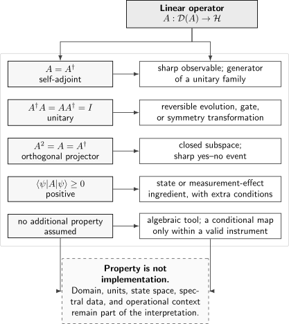
Common operator properties constrain possible physical roles, but context still matters. In particular, being linear does not by itself make an operator an observable or a deterministic state transformation.

Operator as a Linear Map

Unless stated otherwise, operators in the standard state-vector formalism are linear maps. Linearity means

$$A\left(a|\psi\rangle+b|\phi\rangle\right) = aA|\psi\rangle+bA|\phi\rangle$$

whenever $|\psi\rangle,|\phi\rangle\in\mathcal D(A)$ and $a,b\in\mathbb C$. The domain of a linear operator is itself a linear subspace, so the superposition on the left also belongs to the domain.

For an operator on $\mathcal H$, both the input and output lie in the same Hilbert space. More general linear maps can connect different spaces,

$$A:\mathcal H_1\longrightarrow\mathcal H_2.$$

Quantum information also uses maps whose inputs are operators, for example a channel $\mathcal E$ acting on density operators. Such superoperators are linear maps on an operator space, but they are not the primary subject here.

Domain, codomain, and action

A complete specification of an operator records:

1. its domain $\mathcal D(A)$;
2. its codomain;
3. its action on every vector in the domain.

Two formal expressions are not necessarily the same operator if they carry different domains or boundary conditions. Conversely, different-looking formulas can represent the same abstract operator in different bases.

The identity and zero operators illustrate the simplest actions:

$$I|\psi\rangle=|\psi\rangle, \qquad 0|\psi\rangle=0.$$

An operator can carry physical units. Position has dimensions of length, momentum has dimensions of momentum, and a Hamiltonian has dimensions of energy. Consequently, sums such as $A+B$ are physically meaningful only when the terms have compatible dimensions, even if their matrix sizes agree.

Operators Acting on Kets

The expression

$$|\chi\rangle=A|\psi\rangle$$

means: apply $A$ to $|\psi\rangle$ and call the resulting vector $|\chi\rangle$. It does not by itself say that $|\chi\rangle$ is a possible post-measurement state, or even a normalized physical state.

For example, in the basis $\{|0\rangle,|1\rangle\}$, let

$$\begin{aligned} \sigma_x|0\rangle&=|1\rangle,\\ \sigma_x|1\rangle&=|0\rangle. \end{aligned}$$

Linearity then fixes the action on every qubit state:

$$\sigma_x\left(\alpha|0\rangle+\beta|1\rangle\right) = \beta|0\rangle+\alpha|1\rangle.$$

The operator $\sigma_x$ is unitary, so a normalized input gives a normalized output. A general linear operator does not preserve norm:

$$\|A|\psi\rangle\|^2 = \langle\psi|A^\dagger A|\psi\rangle.$$

Only if $A^\dagger A=I$ on the relevant space does this equal $\langle\psi|\psi\rangle$ for every state.

When normalization is meaningful

If $A|\psi\rangle\ne0$, one can form the unit vector

$$|\widetilde\chi\rangle = \frac{A|\psi\rangle} {\sqrt{\langle\psi|A^\dagger A|\psi\rangle}}.$$

This algebraic normalization does not automatically define a physical process. It has an operational meaning when $A$ is supplied as part of a valid state-update rule, such as a measurement operator associated with a selected outcome. In that setting,

$$p(A|\psi\rangle) = \langle\psi|A^\dagger A|\psi\rangle$$

is the outcome probability, provided all outcome operators together satisfy the required completeness relation. See Generalized Measurements: Overview for that larger structure.

Applying an observable is not measuring it

If $A$ represents a sharp observable, $A|\psi\rangle$ is an ordinary vector used in algebraic expressions such as

$$\langle A\rangle_\psi = \langle\psi|A|\psi\rangle.$$

A measurement of $A$ is instead described by its spectral projectors, the Born rule, and a specified state-update model. In general, $A|\psi\rangle$ is not an eigenstate of $A$ and is not the state left after measuring $A$. The distinction between operator action and measurement is foundational, not merely terminological.

An Operator Is Determined by Its Action on a Basis

For a finite-dimensional space with basis $\{|e_n\rangle\}_{n=1}^d$, every state has a unique expansion

$$|\psi\rangle=\sum_{n=1}^d c_n|e_n\rangle.$$

Once the vectors $A|e_n\rangle$ are known, linearity determines

$$A|\psi\rangle = \sum_{n=1}^d c_nA|e_n\rangle.$$

This fact underlies matrix representations: the $n$th matrix column records the components of $A|e_n\rangle$.

In an infinite-dimensional Hilbert space, the same idea requires care. An orthonormal-basis expansion converges in norm, but an unbounded operator need not commute with taking an arbitrary infinite limit. The vector must lie in $\mathcal D(A)$, and convergence of the transformed series must be controlled. The finite-dimensional slogan remains useful, but it does not erase domain questions.

Algebra of Operators

Operators can be combined, but each combination has mathematical and physical conditions.

Sums and scalar multiples

For operators $A$ and $B$,

$$\begin{aligned} (A+B)|\psi\rangle &=A|\psi\rangle+B|\psi\rangle,\\ (\lambda A)|\psi\rangle &=\lambda A|\psi\rangle. \end{aligned}$$

For unbounded operators, the natural domain of the sum is at least $\mathcal D(A)\cap\mathcal D(B)$. A formal sum is of little use if this intersection is not suitable for the intended problem.

Products and order

The product $AB$ means composition:

$$(AB)|\psi\rangle=A\left(B|\psi\rangle\right).$$

The rightmost operator acts first. The vector $|\psi\rangle$ must lie in $\mathcal D(B)$, and $B|\psi\rangle$ must lie in $\mathcal D(A)$. Thus

$$\mathcal D(AB) = \left\lbrace |\psi\rangle\in\mathcal D(B): B|\psi\rangle\in\mathcal D(A) \right\rbrace.$$

Operator multiplication is associative where the compositions are defined, but generally not commutative:

$$AB\ne BA.$$

The difference is the commutator $[A,B]=AB-BA$. Noncommutativity carries physical information about compatibility, transformations, and dynamics.

Powers, inverses, and functions

Powers use repeated composition, $A^2=AA$. An inverse $A^{-1}$ exists only when the relevant map is one-to-one and onto, with suitable domain properties. Eigenvalue zero obstructs an everywhere-defined finite-dimensional inverse.

Exponentials, square roots, resolvents, and other functions of operators are not generally obtained by applying the scalar function to each matrix entry. Their definition comes from power series, diagonalization, or spectral calculus.

Matrix Representation

Choose an orthonormal basis $\{|e_n\rangle\}$. The matrix elements of $A$ are

$$A_{mn}=\langle e_m|A|e_n\rangle.$$

If

$$|\psi\rangle=\sum_n c_n|e_n\rangle,$$

then the output components are

$$\begin{aligned} A|\psi\rangle &=\sum_m c'_m|e_m\rangle,\\ c'_m &=\sum_n A_{mn}c_n. \end{aligned}$$

This is ordinary matrix-vector multiplication. The matrix of a product follows from inserting the identity:

$$\begin{aligned} (AB)_{mn} &=\langle e_m|AB|e_n\rangle\\ &=\sum_k \langle e_m|A|e_k\rangle \langle e_k|B|e_n\rangle\\ &=\sum_k A_{mk}B_{kn}. \end{aligned}$$

The operator is not its matrix

The abstract operator is basis-independent; its entries are not. If a new orthonormal basis is related to the old one by a unitary coordinate change $S$, then a consistent passive change gives

$$[A]'=S^\dagger[A]S, \qquad [\,|\psi\rangle\,]'=S^\dagger[\,|\psi\rangle\,].$$

The transformed matrix and transformed components describe the same geometric action. Keeping the state coordinates fixed while replacing $[A]$ by $S^\dagger[A]S$ generally describes a different calculation.

For a careful separation of active transformations and passive coordinate changes, see Change of Basis. Concrete matrix, differential, and integral-kernel forms are developed in Operator Representations.

Rank-one operators

Given $|u\rangle$ and $|v\rangle$, the outer product

$$A=|u\rangle\langle v|$$

defines a rank-one operator with action

$$A|\psi\rangle = |u\rangle\langle v|\psi\rangle.$$

It first extracts the component along $|v\rangle$, then returns a multiple of $|u\rangle$. Its range is contained in the span of $|u\rangle$, and

$$A^\dagger=|v\rangle\langle u|.$$

When $|u\rangle=|v\rangle$ is normalized, $A$ is the orthogonal projector onto that one-dimensional subspace.

Beyond Matrices

An infinite-dimensional operator may be represented by a differential expression, a multiplication rule, or an integral kernel.

In the position representation on the line,

$$(\hat x\psi)(x)=x\psi(x),$$

while momentum has the formal differential action

$$(\hat p\psi)(x) = -i\hbar\frac{d\psi}{dx}.$$

An integral operator may act as

$$(A\psi)(x) = \int_{\mathbb R} A(x,x')\psi(x')\,dx'.$$

Here $A(x,x')=\langle x|A|x'\rangle$ is an integral kernel in a generalized position basis. It is a representation of the operator, not a second operator living independently of the abstract map.

The same operator can look radically different in another representation. For example, momentum is differential in position space but multiplicative in momentum space:

$$(\hat p\,\widetilde\psi)(p) = p\,\widetilde\psi(p).$$

The Adjoint

The adjoint $A^\dagger$ is defined through the inner product. For bounded operators on a Hilbert space,

$$\langle\phi|A|\psi\rangle = \langle A^\dagger\phi|\psi\rangle$$

for every $|\phi\rangle$ and $|\psi\rangle$. In a finite-dimensional orthonormal basis, the adjoint is represented by the conjugate transpose:

$$[A^\dagger]=[A]^\dagger, \qquad (A^\dagger)_{mn}=A_{nm}^*.$$

Useful algebraic rules include

$$\begin{aligned} (A+B)^\dagger&=A^\dagger+B^\dagger,\\ (\lambda A)^\dagger&=\lambda^*A^\dagger,\\ (AB)^\dagger&=B^\dagger A^\dagger. \end{aligned}$$

The order reverses in the last line because the adjoint reverses composition. The identity

$$\|A|\psi\rangle\|^2 = \langle\psi|A^\dagger A|\psi\rangle$$

is one reason $A^\dagger A$ appears throughout quantum mechanics.

For an unbounded operator, the adjoint has its own domain, $\mathcal D(A^\dagger)$, determined by which vectors make the defining inner product relation continuous in the required sense. Formal conjugation or integration by parts is only the beginning. The canonical mathematical treatment is Adjoint Operators.

Hermitian and Self-Adjoint Operators

In finite dimension, a Hermitian operator satisfies

$$A^\dagger=A.$$

It has real eigenvalues, orthogonal eigenspaces for distinct eigenvalues, and an orthonormal eigenbasis. For every normalized state,

$$\begin{aligned} \langle A\rangle_\psi^* &=\langle\psi|A^\dagger|\psi\rangle\\ &=\langle\psi|A|\psi\rangle, \end{aligned}$$

so its expectation value is real.

Every $2\times2$ Hermitian matrix can be written

$$A=a_0I+a_x\sigma_x+a_y\sigma_y+a_z\sigma_z, \qquad a_\mu\in\mathbb R.$$

This expansion is especially useful for qubits: the identity fixes a common offset, while the real vector $(a_x,a_y,a_z)$ fixes the distinguished Bloch axis.

In infinite-dimensional analysis, self-adjoint is the precise condition

$$A=A^\dagger$$

including equality of domains. The weaker condition often called Hermitian or symmetric requires only

$$\langle\phi|A|\psi\rangle = \langle A\phi|\psi\rangle$$

for vectors in $\mathcal D(A)$. A symmetric operator need not be self-adjoint. Standard sharp observables are represented by self-adjoint operators, not by bare differential expressions. See Hermitian vs Self-Adjoint Operators for the focused distinction and Hermitian Operators for the finite-dimensional facts.

Unitary Operators

An operator $U$ is unitary when

$$U^\dagger U=UU^\dagger=I.$$

Equivalently, $U^{-1}=U^\dagger$. A unitary operator preserves inner products:

$$\langle U\phi|U\psi\rangle = \langle\phi|\psi\rangle.$$

It therefore preserves norms, angles, orthogonality, and transition probabilities:

$$\left|\langle U\phi|U\psi\rangle\right|^2 = \left|\langle\phi|\psi\rangle\right|^2.$$

These invariances make unitaries the appropriate operators for deterministic closed-system evolution and ideal reversible gates. For example,

$$U(t)=e^{-iHt/\hbar}$$

is unitary when $H$ is self-adjoint. The detailed dynamical meaning belongs to The Time-Evolution Operator.

A unitary change of basis and a physical unitary transformation use the same algebra but answer different questions. In a passive basis change, the coordinates change while the abstract state does not. In an active transformation, the physical ray changes relative to a fixed reference frame. Context determines which reading is intended.

See Unitary Operators for their general linear-algebra properties.

Projection Operators

An orthogonal projector $P$ satisfies

$$P^2=P, \qquad P^\dagger=P.$$

Every vector decomposes as

$$|\psi\rangle = P|\psi\rangle+(I-P)|\psi\rangle,$$

and the two terms are orthogonal:

$$\langle\psi|P(I-P)|\psi\rangle=0.$$

The range of $P$ is the selected subspace, while its kernel is the orthogonal complement. If $P$ represents a sharp yes-no event and $|\psi\rangle$ is normalized, the yes probability is

$$p_{\mathrm{yes}} = \langle\psi|P|\psi\rangle = \|P|\psi\rangle\|^2.$$

If the yes outcome is obtained in the simplest projective update model, the conditional state is

$$|\psi_{\mathrm{yes}}\rangle = \frac{P|\psi\rangle} {\sqrt{\langle\psi|P|\psi\rangle}},$$

provided $p_{\mathrm{yes}}>0$. The canonical physical treatment is Projectors; the underlying linear algebra is summarized in Projectors.

Positive and Normal Operators

An operator $A$ is positive, written $A\ge0$, when

$$\langle\psi|A|\psi\rangle\ge0$$

for every vector in its domain. In finite dimension, positivity implies Hermiticity and nonnegative eigenvalues. Every operator of the form $B^\dagger B$ is positive because

$$\langle\psi|B^\dagger B|\psi\rangle = \|B|\psi\rangle\|^2\ge0.$$

Positive operators occur in several roles:

• A density operator is positive and has unit trace.
• A measurement effect $E$ satisfies $0\le E\le I$.
• A positive Hamiltonian has energy bounded below by zero under the chosen energy convention.
• The operator $A^\dagger A$ controls norms and singular values.

These uses are not interchangeable. A density operator is not automatically a measurement effect in an operational model, even if its spectrum happens to lie between zero and one.

An operator is normal when

$$A^\dagger A=AA^\dagger.$$

Self-adjoint and unitary operators are normal. Finite-dimensional normal operators admit an orthonormal eigenbasis, while a generic operator need not. The mathematical details live at Normal Operators.

Transformations, Generators, and Observables

A useful discipline is to distinguish an infinitesimal generator from the finite transformation it generates. If $G$ is self-adjoint and $\theta$ is a real parameter with compatible units, then

$$U(\theta) = \exp\left(-\frac{i\theta G}{\kappa}\right)$$

is unitary, where $\kappa$ supplies the units needed to make the exponent dimensionless.

For an infinitesimal parameter change,

$$U(\delta\theta) = I-\frac{i\,\delta\theta}{\kappa}G +O(\delta\theta^2).$$

The roles differ:

• $G$ is the generator and often also represents an observable.
• $U(\theta)$ is the finite transformation.
• $G|\psi\rangle$ is neither the transformed state nor a measurement outcome.

Examples include the Hamiltonian generating time translations, momentum generating spatial translations, and angular momentum generating rotations. The connection between generators and conserved observables requires the dynamical and symmetry assumptions stated in their canonical chapters.

Spectra and Operator Functions

If a nonzero vector satisfies

$$A|a\rangle=a|a\rangle,$$

then $|a\rangle$ is an eigenvector and $a$ is an eigenvalue. This is one way an operator can act especially simply, but it is not the definition of an operator. Some operators have continuous spectrum, some have both discrete and continuous parts, and nonnormal finite matrices need not possess a complete orthonormal eigenbasis.

For a self-adjoint operator, the spectral theorem provides a projection-valued decomposition. In a purely discrete case,

$$A=\sum_a aP_a.$$

The same projectors define functions,

$$f(A)=\sum_a f(a)P_a,$$

and the sharp measurement probabilities

$$\Pr(A=a\,|\,\psi) = \langle\psi|P_a|\psi\rangle.$$

This is why the operator’s physical meaning as an observable is carried by its full spectral measure, not by a list of eigenvalues alone. Continue with Eigenvalues and Eigenstates, Discrete and Continuous Spectra, and Spectral Theorem: Practical Form.

Operators on Composite Systems

For a bipartite Hilbert space

$$\mathcal H_{AB} = \mathcal H_A\otimes\mathcal H_B,$$

an operator acting only on subsystem $A$ is represented as

$$A_{\mathrm{local}}=A\otimes I_B.$$

Its action on a product vector is

$$(A\otimes I_B) \left(|\psi\rangle_A\otimes|\phi\rangle_B\right) = \left(A|\psi\rangle_A\right)\otimes|\phi\rangle_B.$$

Similarly, $A\otimes B$ acts on both factors. Operators on different factors commute:

$$[A\otimes I_B,I_A\otimes B]=0.$$

This algebraic fact does not imply that every pair of observables in a composite experiment is statistically independent. Entangled states can have correlated local outcomes even when the corresponding local operators commute. See Subsystems and Local Observables for the physical interpretation.

Operators in Infinite-Dimensional Spaces

Every operator on a finite-dimensional Hilbert space is bounded and defined on the whole space. In infinite dimension, bounded and unbounded operators behave differently.

A bounded operator satisfies

$$\|A\psi\|\le C\|\psi\|$$

for some finite $C$ and every $\psi\in\mathcal H$. It extends continuously to the whole Hilbert space. The canonical definition and examples are in Bounded Operators.

An unbounded operator has no such global bound. Position and momentum on $L^2(\mathbb R)$ are standard examples. Their natural domains are proper dense subspaces:

$$\mathcal D(\hat x) = \left\lbrace \psi\in L^2(\mathbb R): x\psi(x)\in L^2(\mathbb R) \right\rbrace,$$

and a common self-adjoint realization of momentum has

$$\mathcal D(\hat p) = \left\lbrace \psi\in L^2(\mathbb R): \psi\text{ is suitably absolutely continuous and } \psi'\in L^2(\mathbb R) \right\rbrace.$$

The phrase “suitably absolutely continuous” suppresses technical equivalence classes that the rigorous toolkit makes precise. The important formalism-level lesson is that neither differential expression acts on every square-integrable function.

Boundary conditions change the operator

On an interval, the same differential expression

$$-i\hbar\frac{d}{dx}$$

can acquire different domains through boundary conditions. Periodic and quasiperiodic conditions, for example, lead to distinct self-adjoint momentum operators with different spectra. The formula alone therefore does not determine the physical operator.

Formal algebra can fail on domains

For unbounded $A$ and $B$, the products $AB$ and $BA$ can have different domains, and their common domain may be too small for a proposed commutator identity. Likewise, an apparent integration-by-parts proof may hide boundary terms. Before manipulating an unbounded operator, ask:

1. Is the vector in the operator’s domain?
2. Does each intermediate result lie in the next operator’s domain?
3. Are the adjoint and boundary conditions specified?
4. Is the claimed equality an operator equality, a quadratic-form identity, or only a formal differential identity?

The rigorous canonical homes are Unbounded Operators and Domains of Operators.

Worked Example: A Rank-One Map

Let $|u\rangle$ and $|v\rangle$ be normalized but not necessarily orthogonal, and define

$$A=|u\rangle\langle v|.$$

The action is

$$A|\psi\rangle = \langle v|\psi\rangle\,|u\rangle.$$

Therefore,

$$\begin{aligned} A^\dagger A &=|v\rangle\langle u|u\rangle\langle v|\\ &=|v\rangle\langle v|,\\ AA^\dagger &=|u\rangle\langle u|. \end{aligned}$$

Several conclusions follow:

• $A$ preserves neither arbitrary norms nor arbitrary inner products.
• $A$ is normal exactly when the projectors onto $|u\rangle$ and $|v\rangle$ agree, which for normalized vectors means the rays agree.
• $A$ is Hermitian only when its phase convention makes $|u\rangle\langle v|=|v\rangle\langle u|$.
• $A$ becomes a rank-one orthogonal projector when $|u\rangle=|v\rangle$.

The example shows how adjoints and products reveal an operator’s role more reliably than its notation.

Worked Example: Matrix, Basis Action, and Units

In the energy basis $\{|0\rangle,|1\rangle\}$ of a two-level model, take

$$H= \begin{pmatrix} E_0 & g\\ g^* & E_1 \end{pmatrix}, \qquad E_0,E_1\in\mathbb R.$$

The entries all have dimensions of energy. Its action on the basis is read from the columns:

$$\begin{aligned} H|0\rangle&=E_0|0\rangle+g^*|1\rangle,\\ H|1\rangle&=g|0\rangle+E_1|1\rangle. \end{aligned}$$

Because $H^\dagger=H$, it can represent a Hamiltonian. For

$$|\psi\rangle=\alpha|0\rangle+\beta|1\rangle,$$

the vector $H|\psi\rangle$ is

$$H|\psi\rangle = \left(E_0\alpha+g\beta\right)|0\rangle +\left(g^*\alpha+E_1\beta\right)|1\rangle.$$

This vector is generally not normalized and does not represent “the state after measuring the energy.” Its uses include evaluating the expectation $\langle\psi|H|\psi\rangle$ and entering the Schrödinger equation.

Worked Example: Differential Adjoint and Boundary Terms

Take the formal momentum expression on an interval $[0,L]$:

$$\hat p=-i\hbar\frac{d}{dx}.$$

For sufficiently regular functions,

$$\begin{aligned} \langle\phi|\hat p\psi\rangle &= \int_0^L \phi^*(x) \left(-i\hbar\psi'(x)\right)\,dx\\ &= \int_0^L \left(-i\hbar\phi'(x)\right)^* \psi(x)\,dx\\ &\quad -i\hbar \left[\phi^*(x)\psi(x)\right]_0^L. \end{aligned}$$

The first integral has the desired formal adjoint action. The boundary term decides whether the operator is symmetric on a proposed domain. Periodic conditions make it vanish for pairs of periodic functions; other boundary conditions require separate analysis. This calculation explains why “take the complex-conjugate transpose” is not a complete prescription for differential operators.

A Practical Operator Audit

When an unfamiliar operator appears, identify the following before calculating:

1. Space: What Hilbert space, tensor factor, or operator space does it act on?
2. Domain: Is it everywhere defined and bounded, or is a proper domain required?
3. Action: Is it given abstractly, by basis action, by a matrix, by a kernel, or by a differential expression?
4. Representation: Which basis or coordinates are being used?
5. Units: What dimensions do its matrix elements, parameters, and eigenvalues carry?
6. Adjoint property: Is it self-adjoint, unitary, positive, normal, projective, or none of these?
7. Physical role: Is it an observable, a finite transformation, a generator, a state, an effect, an outcome operator, or an algebraic aid?
8. Operational context: If it maps states to states, what guarantees positivity, normalization, or an associated success probability?
9. Spectral assumptions: Is a discrete eigenbasis actually available, or is continuous-spectrum machinery needed?
10. Composition: Are products and commutators defined on the vectors being used?

This audit prevents most category errors before they become algebraic errors.

Common Mistakes

• Treating the matrix as basis-free. A matrix represents an operator only after bases for its input and output spaces are fixed.
• Reading $A|\psi\rangle$ as a measurement. Operator action is an algebraic operation; measurement needs a probability and state-update rule.
• Assuming every operator maps normalized states to normalized states. Norm preservation is a special property, not a consequence of linearity.
• Renormalizing without an operational model. Any nonzero vector can be normalized, but that does not make the nonlinear rule physically valid.
• Confusing a generator with its finite transformation. $H$ and $e^{-iHt/\hbar}$ have different properties and roles.
• Using “Hermitian” as a universal synonym for observable. Sharp observables require self-adjoint operators; generalized observables use POVMs.
• Assuming real eigenvalues imply Hermiticity. A nonnormal matrix can have real eigenvalues without being Hermitian.
• Assuming diagonalizable means unitarily diagonalizable. The latter requires normality in finite dimension.
• Dropping identity factors on composite systems ambiguously. Write $A\otimes I$ until the subsystem convention is unambiguous.
• Ignoring domains. A differential formula, boundary condition, and domain together define the operator.
• Reversing composition order. In $AB|\psi\rangle$, $B$ acts first.
• Applying scalar functions entrywise. Operator functions are defined by algebraic or spectral calculus, not generally element by element.

Interpretation Boundary

Operators organize the predictive formalism, but an abstract operator does not by itself specify a laboratory device. A self-adjoint operator determines the outcome statistics of an ideal sharp observable together with a state and the Born rule. It does not uniquely determine the physical coupling, detector design, measurement duration, disturbance, or readout noise.

Likewise, knowing that a map is linear is not enough to make it a possible quantum evolution. Deterministic evolution of density operators must obey positivity, trace preservation, and the appropriate extension to composite systems. State-vector unitaries are one important special case. Keeping mathematical type, operator property, and physical implementation distinct is part of using the formalism precisely.

Summary

• An operator is specified by its spaces, domain, and action.
• Standard state-vector operators are linear, but linearity alone fixes no physical interpretation.
• The expression $A|\psi\rangle$ is an operator action, not automatically a measurement or a normalized state.
• Matrices, differential expressions, and kernels are representations of operators.
• The adjoint organizes norm, expectation, self-adjointness, unitarity, positivity, and projection.
• Self-adjoint operators represent standard sharp observables; unitary operators represent reversible transformations; projectors represent subspaces and sharp events.
• Products act right to left and may be order-dependent.
• In infinite dimension, domains and boundary conditions are part of the operator and cannot be suppressed safely.

References

• P. A. M. Dirac, The Principles of Quantum Mechanics, 4th ed., Oxford University Press, 1958, Chapters I–III.
• J. von Neumann, Mathematical Foundations of Quantum Mechanics, Princeton University Press, 1955, Chapters II–III.
• R. Shankar, Principles of Quantum Mechanics, 2nd ed., Springer, 1994, Chapters 1 and 4.
• J. J. Sakurai and J. Napolitano, Modern Quantum Mechanics, 3rd ed., Cambridge University Press, 2020, Chapter 1.
• B. C. Hall, Quantum Theory for Mathematicians, Springer, 2013, Chapters 2–4.
• M. Reed and B. Simon, Methods of Modern Mathematical Physics, Volume I: Functional Analysis, revised and enlarged ed., Academic Press, 1980.
• M. Nielsen and I. Chuang, Quantum Computation and Quantum Information, 10th anniversary ed., Cambridge University Press, 2010, Sections 2.1–2.2.
• J. Weidmann, Linear Operators in Hilbert Spaces, Springer, 1980.

Exercises

Exercise 1: Reconstruct an operator from basis action

In an orthonormal basis $\{|0\rangle,|1\rangle\}$, an operator satisfies

$$\begin{aligned} A|0\rangle&=2|0\rangle-i|1\rangle,\\ A|1\rangle&=3|0\rangle+|1\rangle. \end{aligned}$$

Find its matrix and compute $A(\alpha|0\rangle+\beta|1\rangle)$.

Solution

The basis images form the matrix columns:

$$[A]= \begin{pmatrix} 2 & 3\\ -i & 1 \end{pmatrix}.$$

By linearity,

$$\begin{aligned} A(\alpha|0\rangle+\beta|1\rangle) &=\alpha A|0\rangle+\beta A|1\rangle\\ &=(2\alpha+3\beta)|0\rangle +(-i\alpha+\beta)|1\rangle. \end{aligned}$$

Exercise 2: Operator order

Let

$$\sigma_x= \begin{pmatrix} 0&1\\ 1&0 \end{pmatrix}, \qquad \sigma_z= \begin{pmatrix} 1&0\\ 0&-1 \end{pmatrix}.$$

Compute $\sigma_x\sigma_z|0\rangle$ and $\sigma_z\sigma_x|0\rangle$. What does the result say about order?

Solution

Because the rightmost operator acts first,

$$\begin{aligned} \sigma_x\sigma_z|0\rangle &=\sigma_x|0\rangle=|1\rangle,\\ \sigma_z\sigma_x|0\rangle &=\sigma_z|1\rangle=-|1\rangle. \end{aligned}$$

Thus the products act differently:

$$\sigma_x\sigma_z|0\rangle = -\sigma_z\sigma_x|0\rangle.$$

Indeed, the two Pauli matrices anticommute and do not commute.

Exercise 3: Adjoint and norm change

For

$$A= \begin{pmatrix} 1&1\\ 0&1 \end{pmatrix},$$

find $A^\dagger A$. Does $A$ preserve the norm of every vector? Test the normalized state $|1\rangle$.

Solution

The adjoint and product are

$$A^\dagger= \begin{pmatrix} 1&0\\ 1&1 \end{pmatrix}, \qquad A^\dagger A= \begin{pmatrix} 1&1\\ 1&2 \end{pmatrix}.$$

Since $A^\dagger A\ne I$, the operator is not unitary and does not preserve every norm. In particular,

$$A|1\rangle=|0\rangle+|1\rangle,$$

whose squared norm is $2$, not $1$.

Exercise 4: Rank-one operator

For normalized vectors $|u\rangle$ and $|v\rangle$, set $A=|u\rangle\langle v|$. Show that $A^\dagger A$ is a projector. Under what condition is $A$ itself a projector?

Solution

First,

$$A^\dagger=|v\rangle\langle u|.$$

Normalization of $|u\rangle$ gives

$$A^\dagger A = |v\rangle\langle u|u\rangle\langle v| = |v\rangle\langle v|.$$

This is the rank-one orthogonal projector onto the ray of $|v\rangle$.

For $A$ itself to be an orthogonal projector, it must satisfy both $A^\dagger=A$ and $A^2=A$. These conditions hold when $|u\rangle$ and $|v\rangle$ represent the same ray with phases chosen so that $A=|v\rangle\langle v|$. Equivalently, the operator itself must reduce to a normalized rank-one projector.

Exercise 5: Projected components

Let $P$ be an orthogonal projector and $Q=I-P$. Prove that $P|\psi\rangle$ and $Q|\psi\rangle$ are orthogonal, and derive

$$\|\psi\|^2 = \|P\psi\|^2+\|Q\psi\|^2.$$

Solution

Since $P^\dagger=P$ and $P^2=P$,

$$\begin{aligned} \langle P\psi|Q\psi\rangle &=\langle\psi|P(I-P)|\psi\rangle\\ &=\langle\psi|(P-P^2)|\psi\rangle\\ &=0. \end{aligned}$$

Also, $|\psi\rangle=P|\psi\rangle+Q|\psi\rangle$. The two terms are orthogonal, so the Pythagorean identity gives

$$\|\psi\|^2 = \|P\psi\|^2+\|Q\psi\|^2.$$

Exercise 6: Generator versus transformation

Suppose $G=G^\dagger$ and

$$U(\theta)=e^{-i\theta G}.$$

Show directly that $U(\theta)$ is unitary. Then explain why $G|\psi\rangle$ should not be identified with the state $U(\theta)|\psi\rangle$.

Solution

Because $G$ is self-adjoint and $\theta$ is real,

$$U(\theta)^\dagger=e^{i\theta G}.$$

Both exponentials are functions of the same operator and therefore commute:

$$U(\theta)^\dagger U(\theta) = e^{i\theta G}e^{-i\theta G} = I.$$

The same calculation in the opposite order gives $UU^\dagger=I$.

The vector $G|\psi\rangle$ is the action of the infinitesimal generator. The finite transformed state is the full exponential series,

$$U(\theta)|\psi\rangle = \left( I-i\theta G-\frac{\theta^2G^2}{2}+\cdots \right)|\psi\rangle.$$

They are different vectors with different units unless conventions make $\theta G$ dimensionless.

Exercise 7: A local operator

For two qubits, evaluate

$$(\sigma_z\otimes I) \frac{|00\rangle+|11\rangle}{\sqrt2}.$$

Is the result a product state? Does $\sigma_z\otimes I$ commute with $I\otimes\sigma_x$?

Solution

Using $\sigma_z|0\rangle=|0\rangle$ and $\sigma_z|1\rangle=-|1\rangle$,

$$(\sigma_z\otimes I) \frac{|00\rangle+|11\rangle}{\sqrt2} = \frac{|00\rangle-|11\rangle}{\sqrt2}.$$

The output remains entangled and is not a product state.

Operators on different tensor factors commute:

$$\begin{aligned} (\sigma_z\otimes I)(I\otimes\sigma_x) &=\sigma_z\otimes\sigma_x,\\ (I\otimes\sigma_x)(\sigma_z\otimes I) &=\sigma_z\otimes\sigma_x. \end{aligned}$$

Therefore their commutator vanishes.

Exercise 8: Boundary form for momentum

Let $\hat p=-i\hbar\,d/dx$ on $[0,L]$. Starting from integration by parts, show that the boundary obstruction to symmetry is

$$-i\hbar \left[ \phi^*(L)\psi(L)-\phi^*(0)\psi(0) \right].$$

Verify that it vanishes when both functions obey

$$\psi(L)=e^{i\alpha}\psi(0), \qquad \phi(L)=e^{i\alpha}\phi(0)$$

for the same real $\alpha$.

Solution

Integration by parts gives

$$\langle\phi|\hat p\psi\rangle -\langle\hat p\phi|\psi\rangle = -i\hbar \left[ \phi^*(L)\psi(L)-\phi^*(0)\psi(0) \right].$$

Under the stated boundary conditions,

$$\phi^*(L)\psi(L) = e^{-i\alpha}\phi^*(0) e^{i\alpha}\psi(0) = \phi^*(0)\psi(0).$$

The boundary form therefore vanishes. This proves symmetry on the proposed domain. Establishing self-adjointness also requires showing that the adjoint has exactly the same domain.

Exercise 9: Diagnose an invalid inference

A calculation applies

$$A= \begin{pmatrix} 2&0\\ 0&1 \end{pmatrix}$$

to every normalized qubit and then renormalizes the output. Explain why linearity of $A$ does not make this a deterministic closed-system evolution. Give one algebraic and one operational reason.

Solution

Algebraically,

$$A^\dagger A= \begin{pmatrix} 4&0\\ 0&1 \end{pmatrix} \ne I,$$

so $A$ is not unitary and does not preserve all norms or inner products. The subsequent normalization depends on the input state, making the combined map on state vectors nonlinear.

Operationally, a nonunitary outcome operator can describe a selected measurement result only as part of a complete instrument. One must supply a success probability and other outcomes satisfying a completeness relation. The bare instruction “apply and renormalize” supplies neither and therefore does not define a deterministic physical evolution.