Map of the Volume

The volume is organized around a progression from what the system is, through how it is prepared and probed, to which collective structures its observables support. That progression is a dependency map, not a claim that every many-body problem follows one universal algorithm.

Use this page to locate missing prerequisites, choose the correct family of tools, and keep finite-size, ensemble, approximation, and evidence assumptions attached to every conclusion. Use the Reading Paths when you want a course-like sequence optimized for a particular goal.

Required background. Read the volume introduction and Why Many-Body Physics Is Different first. The Core Objects and Notation page supplies the notation used below.

The map at a glance

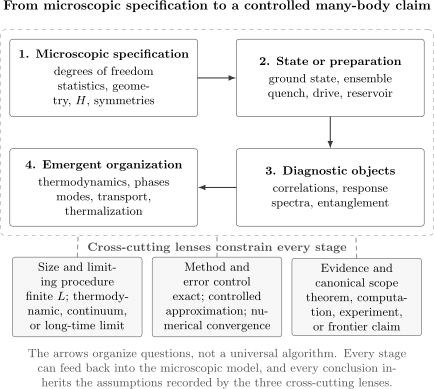
A controlled many-body claim connects microscopic degrees of freedom and a Hamiltonian to a state or preparation, then to diagnostic observables and an emergent description. Size limits, error control, and evidence status constrain every arrow.

Open the vector diagram at full size. The SVG remains sharp under zoom; the complete textual equivalent follows below.

The textual equivalent is:

1. Microscopic specification: degrees of freedom, statistics, geometry, Hilbert space, Hamiltonian, constraints, and symmetries.
2. State or preparation: ground state, excited state, equilibrium ensemble, quench, periodic drive, or coupling to a reservoir.
3. Diagnostic objects: correlation functions, response kernels, spectral functions, entanglement measures, conserved quantities, and order parameters.
4. Emergent organization: thermodynamics, phases, quasiparticles, collective modes, transport, thermalization, or an effective field theory.

Three lenses remain active throughout: the finite-size and limiting procedure, the method and its error control, and the epistemic status and canonical scope of the conclusion.

In compact notation, the spine is

$$(\mathcal H,H) \longrightarrow \rho\ \text{or}\ |\psi\rangle \longrightarrow \{C,\chi,A,S_A,\ldots\} \longrightarrow \text{collective description}.$$

Here $C$ denotes correlations, $\chi$ response, $A$ a spectral function, and $S_A$ an entanglement measure. The arrow does not mean that the later description is automatic: it represents a chain of calculations and controlled inferences whose assumptions must be stated.

Layer 0: reusable prerequisites

Many-body physics applies structures defined elsewhere rather than deriving them again.

Capability	Canonical preparation
density operators and trace expectations	Density Operators
tensor products and local observables	Tensor Products of Hilbert Spaces and Local and Global Observables
identical particles and exchange symmetry	Identical Particles
Fock space and creation–annihilation algebra	Fock Space and Second Quantization
pictures of time evolution and Green functions	Quantum Dynamics
symmetry, conserved quantities, and spin	Symmetry, Angular Momentum, and Spin
perturbative and variational reasoning	Approximation and Semiclassical Methods

The Math Needed for Many-Body QM page gives a finer diagnostic. A spin-system route can begin before Fock space. Particle and quantum-gas routes can begin with symmetrized first-quantized states, but most later operator-based treatments in this volume use Fock space and second quantization as their working language.

Layer 1: scale, kinematics, and statistics

The first internal layer asks how the state space and observables change as the number of degrees of freedom grows.

• Few-Body versus Many-Body Physics separates problem structure, observable-relative macroscopicity, and thermodynamic-limit claims.
• Scaling of Hilbert Space explains exponential and combinatorial growth.
• Locality in Many-Body Systems separates support, interaction arity, geometric range, decay, and dynamical quasi-locality.
• Extensive and Intensive Quantities classifies totals, densities, boundary terms, additivity, and anomalous scaling along a declared family.
• Thermodynamic Limit specifies how that family is taken to infinity and which limits are expected to exist.
• Finite-Size Effects diagnoses spectral quantization, gap identities, boundaries, shells, commensurability, correlation cutoffs, and recurrence windows for realizable finite systems.
• Preview Emergence and Effective Degrees of Freedom here only to recognize that later layers may change variables. Perform its full matching and validation audit in Layer 5, after the model, state, and diagnostic are explicit.
• Many-Body Hilbert Spaces and Operators routes from the declared state space to coordinate, occupation-number, mode-operator, field-operator, observable, and representation choices. For direct lookup, use Occupation-Number Representation or Field Operators.

Exit condition. You can state the Hilbert space, statistics, constraints, complete modes and their ordering, working representation, geometry, boundary conditions, cutoff, and size variable; for each chosen observable, you can also state its normalization, expected leading scaling, subleading terms, whether macroscopic pieces are asymptotically additive, and which finite-size mechanism and resolution scale dominate.

Layer 2: models, interactions, and approximations

The second layer specifies the Hamiltonian or effective dynamical model whose competing terms generate nontrivial many-body behavior.

• Lattice Models and Spin Systems routes from a declared lattice problem to the appropriate spin, particle, impurity, mapping, boundary, or exact-method branch.
• Lattice Models Overview records graph, local-space, coupling, constraint, and boundary data.
• The Transverse-Field Ising Model, Heisenberg Model, Hubbard Model, and Bose–Hubbard Model are recurring laboratories.
• Interacting Systems and Approximation Methods routes from the declared model, regime, target observable, and available control parameter to an approximation family and its validation tests.
• Interacting Many-Body Systems Overview asks which structural assumptions make an approximation plausible.
• Mean-Field Theory and Variational Many-Body States introduce complementary approximation logics.

Exit condition. You can identify the competing terms and dimensionless control parameters, state an exact limit, and explain what correlations an approximation neglects or retains.

Layer 3: state assignments and equilibrium baselines

The third layer chooses a state or ensemble after the state space, Hamiltonian, constraints, and exchanged quantities have been identified. It separates an equilibrium assignment from a dynamical explanation of equilibration.

• Quantum Statistical Mechanics supplies the chapter-level audit from controls and trace domain to equilibrium state, thermodynamic potential, observable, and validity claim.
• Statistical Ensembles Overview compares microcanonical, canonical, and grand-canonical constraints.
• Thermal Density Operators develops Gibbs states and trace expectations.
• Partition Functions and Thermodynamic Potentials connect spectra to thermodynamics.
• Quantum Statistics and Ideal Gases routes from exchange sector and complete modes to occupation laws, ideal-gas models, and regime checks.
• Bose–Einstein Statistics and Fermi–Dirac Statistics establish the noninteracting quantum baselines.
• Ideal Bose Gas and Ideal Fermi Gas turn occupation factors into macroscopic examples.

Exit condition. You can name the state or ensemble, conserved or exchanged quantities, partition function where applicable, and thermodynamic limit, and you can distinguish ensemble weights from Born probabilities.

Layer 4: diagnostics, response, and finite temperature

A model becomes physically useful when it predicts observables and their uncertainty or response.

• Correlation Functions and Linear Response routes a physical question and probe protocol to the appropriate correlation, spectral, susceptibility, sum-rule, or transport branch.
• Correlation Functions Overview distinguishes equal-time, dynamical, connected, ordered, and response correlators.
• Structure Factors and Spectral Functions connect theory to momentum- and frequency-resolved probes.
• Kubo Formula gives the causal linear-response relation after the perturbation and measured observable are fixed.
• Finite-Temperature Methods routes a declared thermal question to the appropriate trace, imaginary-time, Matsubara, spectral, continuation, path-integral, KMS, or real-time branch.
• Finite-Temperature QM Overview gives the integrated roadmap through imaginary time, thermal Green functions, and analytic continuation.
• Fluctuation–Dissipation Theorem relates equilibrium fluctuations to dissipative response under stated conventions.

Exit condition. You can define the operator ordering, connected subtraction, Fourier convention, reference state, and source–response pair for the quantity you intend to calculate.

Layer 5: emergent organization

This layer asks which collective description organizes predictions for selected observables without erasing the evidence that supports it.

• Emergence and Effective Degrees of Freedom supplies the cross-cutting audit for retained and eliminated variables, matching, error, validation, and breakdown.
• Phases, Order, and Criticality routes a proposed macroscopic classification to the appropriate phase-definition, order, symmetry-breaking, transition, scaling, Landau, renormalization-group, or topological-order branch.
• Phases of Matter in Many-Body QM organizes symmetry, order, topology, excitations, and response.
• Quantum Phase Transitions distinguishes zero-temperature quantum critical points from finite-temperature phase transitions and quantum-critical crossovers.
• Quasiparticles and Collective Modes selects the appropriate excitation branch before a specialist calculation or interpretation is attempted.
• Quasiparticles Overview states when particle-like poles and peaks are useful and when they fail.
• Collective Modes develops coherent motion of densities, phases, spins, and other collective coordinates.
• Many-Body Entanglement and Information routes a declared partition and state class to an appropriate information diagnostic, scaling test, representation branch, or operator-growth analysis.
• Many-Body Entanglement Overview records subsystem, state-class, measure, and scaling choices.
• Nonequilibrium Many-Body Dynamics routes a declared preparation, generator, probe, and limit order to the appropriate quench, relaxation, memory, chaos, scrambling, or driven-system branch.
• Nonequilibrium Overview distinguishes equilibration, thermalization, transport, memory, and driven behavior.

Exit condition. You can state the retained and eliminated variables, target observables, matching map, control parameter or empirical error, validation test, and breakdown condition; you can also state what diagnostic distinguishes the proposed organization, which limit makes it sharp, and which alternatives remain compatible with the evidence.

Layer 6: bridge, computation, and lookup

The final layer routes work that changes language or method without changing the underlying physics question.

• Bridges to QFT and Statistical Field Theory routes a declared language change or continuum or effective-theory goal to the appropriate bridge.
• Why Many-Body QM Leads to QFT separates exact second-quantized language, effective collective fields, and full field theory.
• Computational Many-Body QM routes a declared problem, observable, obstruction, and physical limit to the appropriate numerical branch; the Computational Many-Body Overview supplies the detailed method and evidence framework.
• The Model Encyclopedia collects Hamiltonians, limits, observables, and solution status.
• Many-Body and Quantum Statistical Mechanics Reference routes lookup after the conceptual route is known; go directly to Symbols and Conventions when notation or convention translation is the specific task.

Computational QM owns reusable algorithms, implementations, and software validation. Quantum Matter owns material-specific phases and measured phenomenology. QFT.org owns full relativistic and renormalized field-theory developments. The boundary guide makes these handoffs explicit.

Cross-cutting lenses

Finite size and order of limits

A finite calculation is not a defective thermodynamic-limit calculation; it answers a different question. Use Finite-Size Effects to identify spectral, boundary, shell, correlation, commensurability, and recurrence mechanisms. Then record $L$, $N$, geometry, boundary conditions, resolution, and the sequence of limits. A susceptibility peak that sharpens with size may support a transition hypothesis, but one size does not establish a nonanalytic phase transition; numerical extrapolation belongs to Finite-Size Scaling in Numerics.

Locality and interaction range

Locality together with controlled interaction strengths and coordination constrains information propagation. Extensivity, correlation structure, and algorithmic performance additionally depend on the state, spectrum, interaction decay, geometry, and other hypotheses. Long-range interactions can require size-dependent normalization and can change ensemble equivalence or scaling. “Many-body” alone does not determine these properties.

Method and uncertainty

Label a result as exact, perturbative, variational, mean-field, asymptotic, or numerical. For numerical work, report basis truncation, symmetry sector, system sizes, convergence criterion, and an analytic or independent benchmark. Self-consistency is not an error estimate.

Evidence status

Distinguish theorem, controlled approximation, numerical observation, experimental inference, and active conjecture. Frontier ideas such as universal ETH behavior or stable many-body localization require explicit scope conditions; they are not generic consequences of having many degrees of freedom.

Worked route: a Hubbard-chain susceptibility

Suppose the task is to compute the finite-temperature spin susceptibility of a one-dimensional Hubbard chain and compare it with a material measurement.

1. Specify the model. Use the Hubbard Model to define hopping $t$, onsite interaction $U$, filling, chain length, and boundary conditions.
2. Specify the state. Choose canonical or grand-canonical equilibrium and state whether particle number and magnetization are fixed.
3. Specify the response. Use Susceptibilities and the Kubo Formula to define the magnetic source and response observable.
4. Specify the method. A small-chain exact calculation is a finite-size benchmark. A reusable Lanczos, finite-temperature tensor-network, or Monte Carlo implementation belongs in Computational QM and requires convergence evidence.
5. Separate the material comparison. Parameter extraction, lattice chemistry, probe calibration, and interpretation of a named material belong in Quantum Matter.

The calculation is not controlled until all five statements are visible. The map therefore routes assumptions as well as topics.

Common map-reading errors

Treating the arrows as irreversible. Observed spectra can force a revised Hamiltonian, and an emergent theory can reveal which microscopic terms are relevant. The map is iterative.

Assuming every branch is required. A ground-state spin-chain calculation may not need grand-canonical ensembles. An ideal gas may not need lattice models. Use exit conditions to skip mastered or irrelevant branches.

Choosing a method before an observable. No numerical method is best in isolation. Its suitability depends on dimensionality, entanglement, sign structure, temperature, time scale, and required error.

Crossing a canonical boundary silently. A generic model, its material realization, its experimental protocol, and its numerical implementation may occupy four volumes. Link them; do not merge their scopes.

Exercises

Place three systems on the map

For each system, identify the first internal layer and one later diagnostic: (a) an ideal trapped Fermi gas, (b) a zero-temperature Heisenberg chain, and (c) a driven Bose–Hubbard lattice.

Solution

(a) Begin with quantum statistics and the equilibrium baseline; occupation, density profile, or compressibility can be a later diagnostic. (b) Begin with the spin Hilbert space and lattice Hamiltonian; correlations, excitation spectra, entanglement, or an order parameter can diagnose the state. (c) Begin with bosonic Fock space and the Bose–Hubbard Hamiltonian, then specify the drive and initial state; time-dependent correlations, heating, transport, or Floquet observables are possible diagnostics.

Choose a route for a local quench

A local spin is rotated in the middle of an interacting chain, and the goal is to determine how the disturbance spreads. Trace a defensible route through the map before choosing a numerical method.

Solution

Begin with the spin Hilbert space, chain geometry, boundaries, and local Hamiltonian, then specify the initial state and the local rotation as a quench protocol. Choose diagnostics such as time-dependent connected correlations, commutators, or an operator-spreading measure, including their spatial support and time range. Only then select a method compatible with the geometry, entanglement growth, system size, and required error. Compare the observed front with the model’s locality assumptions and the Lieb–Robinson bound without identifying the bound velocity with the measured propagation velocity.

Separate method from physics

Why does “use DMRG” not identify a complete route through the map?

Solution

DMRG names a method, not the Hilbert space, Hamiltonian, state, observable, limit, or physical claim. One must still specify those objects and explain why a matrix-product-state approximation is suitable—for example, because the target is a low-entanglement one-dimensional state—and report truncation and convergence diagnostics. The method implementation belongs in Computational QM; the model and physical interpretation remain in their canonical volumes.

References

• A. Altland and B. Simons, Condensed Matter Field Theory, 2nd ed., Cambridge University Press (2010) — collective fields, response, path integrals, and renormalization interfaces.
• P. Coleman, Introduction to Many-Body Physics, Cambridge University Press (2015) — a graduate-level map from second quantization through response, broken symmetry, and path integrals.
• L. D’Alessio, Y. Kafri, A. Polkovnikov, and M. Rigol, “From quantum chaos and eigenstate thermalization to statistical mechanics and thermodynamics”, Advances in Physics 65, 239–362 (2016) — isolated-system thermalization, ETH, integrability, and their limitations.
• J. Eisert, M. Cramer, and M. B. Plenio, “Area laws for the entanglement entropy”, Reviews of Modern Physics 82, 277–306 (2010) — locality, entanglement scaling, and efficient state representations under stated assumptions.
• G. D. Mahan, Many-Particle Physics, 3rd ed., Springer (2000) — Green functions, spectral methods, response, and interacting applications.
• R. K. Pathria and P. D. Beale, Statistical Mechanics, 3rd ed., Academic Press (2011) — ensembles, thermodynamic limits, quantum statistics, and fluctuations.
• S. Sachdev, Quantum Phase Transitions, 2nd ed., Cambridge University Press (2011) — quantum phases, scaling, universality, and finite-temperature crossovers.