Locality in Many-Body Systems

Locality says where an operator acts and how that support is arranged in physical space or on an interaction graph. It does not mean a small Hilbert space, weak coupling, easy computation, relativistic causality, or locality in the Bell-theorem sense.

A useful locality claim must combine four ledgers:

1. a subsystem decomposition or local observable algebra;
2. a physical metric or graph;
3. the support and strength of every relevant term;
4. the range or decay of couplings along a growing family of systems.

Leaving out any one can turn “the Hamiltonian is local” into an ambiguous slogan. A pair term connecting opposite ends of a chain is two-body but geometrically long-ranged. An onsite Hubbard interaction is quartic in fermion operators but spatially local. A global magnetization is a sum of local densities but is not itself a local observable.

Required background. Review Tensor Products of Hilbert Spaces and Commutators and Anticommutators. The chapter Overview and Scaling of Hilbert Space are helpful but not required.

Support, Range, and Interaction Arity Are Different

Three common meanings of “local” answer different questions.

Property	Definition	Question answered
operator support	the subsystems on which an operator acts nontrivially	where does the operation act?
interaction arity	an upper bound $\lvert X\rvert\le k$ on the number of subsystems in one term	how many factors participate in one term?
geometric range	an upper bound or decay law for $\operatorname{diam}(X)$	how far apart can those factors be?

A complete statement also records the term norms and how many terms touch a site. A Hamiltonian can be two-local yet connect every pair of sites. Dividing its couplings by system size may restore an extensive energy scale, but it does not restore geometric locality.

Operator Support and Physical Geometry

Consider a finite set of sites or subsystems $\Lambda$ with

$$\mathcal H_\Lambda = \bigotimes_{i\in\Lambda} \mathcal h_i.$$

An operator supported on $X\subseteq\Lambda$ has the form

$$O_X = O_X^{(X)} \otimes I_{\Lambda\setminus X}.$$

The support $\operatorname{supp}(O)$ is the smallest such $X$. For ordinary spin or qudit tensor factors, operators with disjoint supports commute:

$$X\cap Y=\varnothing \quad\Longrightarrow\quad [A_X,B_Y]=0.$$

Support alone supplies no distance. The model must also declare a metric $d(i,j)$, usually Euclidean distance, graph distance, or distance inherited from a physical embedding. For sets $X$ and $Y$, define

$$\begin{aligned} d(X,Y) &= \min_{i\in X,\,j\in Y}d(i,j), \\ \operatorname{diam}(X) &= \max_{i,j\in X}d(i,j). \end{aligned}$$

Along a sequence of larger systems, a local observable normally has support size and diameter bounded independently of the total system size. Its location may change with the system—for example, a one-site observable kept near the center—but its physical support does not grow with the volume.

Fermionic locality

Odd fermionic operators on disjoint regions anticommute rather than commute. The physically relevant local observable algebras are normally built from parity-even operators, for which separated regions recover the expected commuting structure. A Jordan–Wigner mapping can turn a local fermionic operator into a long Pauli string; that representation-dependent string does not, by itself, redefine the underlying physical geometry.

The full measurement distinction among local, joint, and global observables belongs to Local and Global Observables.

Interaction Arity Is Not Spatial Range

A lattice Hamiltonian can be decomposed as

$$H_\Lambda = \sum_{X\subseteq\Lambda} h_X,$$

where $h_X$ is supported on $X$.

• It is $k$-local if $|X|\le k$ for every nonzero term.
• It has finite geometric range $R$ if $h_X=0$ whenever $\operatorname{diam}(X)>R$.
• It is short-range or quasi-local more generally when longer terms are allowed but their norms decay sufficiently fast according to a stated condition.

A four-site plaquette term has arity four but can remain geometrically local as the lattice grows. A term $Z_1Z_L$ has arity two but its diameter grows with the length of an open chain. “Few-body interaction” therefore does not mean “few-body system,” and low polynomial degree in creation and annihilation operators does not determine spatial range.

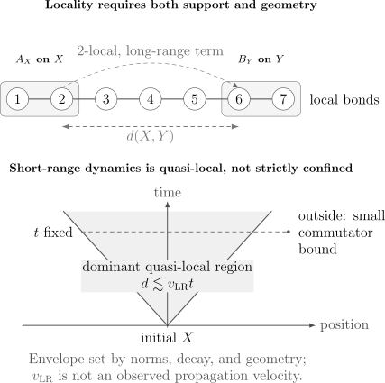
Support, arity, and range are separate data. The upper panel contrasts short-range bonds with a two-site term spanning distant regions. The lower panel depicts a Lieb–Robinson envelope: short-range evolution is quasi-local, but the generic bound permits exponentially small tails outside the effective cone rather than imposing strict zero support.

Finite-Range, Decaying, and Long-Range Hamiltonians

Range is not enough unless interaction strength and coordination remain controlled. A useful finite-system audit quantity is

$$J_* = \sup_{i\in\Lambda} \sum_{X\ni i} \lVert h_X\rVert.$$

For a regular family of bounded-degree, finite-range spin models, $J_*$ remains bounded as $|\Lambda|$ grows. Rigorous quasi-locality theorems use conditions of this kind, often with distance-dependent weights and more precise assumptions.

For pair interactions on a $d$-dimensional lattice, a power-law model may satisfy

$$\lVert h_{ij}\rVert \le \frac{J} {[1+d(i,j)]^\alpha}.$$

Every term is two-local, but the Hamiltonian is not finite-range for any finite $\alpha$. On a regular lattice, the sum of pair strengths incident on a site behaves schematically like

$$\sum_{r=1}^{L} r^{d-1-\alpha}.$$

This sum converges as $L\to\infty$ when $\alpha>d$. For slower decay, a size-dependent Kac or mean-field normalization is often introduced when an extensive energy is desired. That normalization changes the strength ledger, not the geometric fact that distant sites interact directly.

Propagation bounds for long-range interactions depend on $\alpha$, dimension, geometry, norm, and theorem hypotheses. One must not apply a finite-range linear light-cone formula unchanged to a Coulomb, dipolar, cavity-mediated, or all-to-all model.

Spatial Locality in Continuum Systems

Particle labels are not spatial regions. For identical particles, spatial locality is expressed naturally through fields or smeared density operators. A smeared observable

$$A(f) = \int d^d x\, f(\mathbf x) \mathcal O(\mathbf x)$$

is associated with the spatial support of the test function $f$.

A two-particle interaction can be written schematically as

$$H_{\mathrm{int}} = \frac{1}{2} \int d^d x\,d^d y\, V(\mathbf x-\mathbf y) \psi^\dagger(\mathbf x) \psi^\dagger(\mathbf y) \psi(\mathbf y) \psi(\mathbf x).$$

Its spatial range is set by $V$, not by the fact that the term contains two creation and two annihilation operators. For bosons or suitable multicomponent fermions, a contact model replaces the potential by an effective delta interaction and yields a local density such as

$$H_{\mathrm{contact}} = \frac{g}{2} \int d^d x\, \psi^\dagger(\mathbf x) \psi^\dagger(\mathbf x) \psi(\mathbf x) \psi(\mathbf x).$$

Continuum fields are operator-valued distributions, local bosonic spaces may be unbounded, and contact interactions can require regularization and renormalization. Standard bounded-spin lattice theorems therefore do not transfer automatically. For identical spinless fermions, the same-component zero-range $s$-wave term vanishes by antisymmetry; derivative interactions, finite range, or additional internal components require their own operator structure. Real-Space Representation owns the continuum normalization and discretization details.

Local Observables and Global Sums

An onsite density $n_i$ is local. A correlator $n_i n_j$ has support $\{i,j\}$; it is two-local in arity, but its diameter is $d(i,j)$. A block magnetization has support on the block. The total magnetization

$$M = \sum_{i\in\Lambda}m_i$$

is a global observable built from local densities.

This distinction matters twice. First, a global Hamiltonian can be assembled from local terms. Second, a local probe can approach bulk behavior before a global gap, total fluctuation, or long-range correlator does. Extensive and Intensive Quantities owns how sums and densities scale with volume; locality only identifies their support structure.

A Worked Locality Audit

The same algebraic adjectives can hide different geometries.

Model term	Arity	Geometric range	Strength and overlap	Locality conclusion
nearest-neighbor chain, $-JZ_jZ_{j+1}$	two	one edge	$O(1)$ terms touch each site	finite-range on the chain
complete-graph Ising, $-(J/L)Z_iZ_j$	two	up to the system diameter	$L-1$ terms touch each site; $1/L$ controls energy scaling	normalized but geometrically all-to-all
plaquette term, $KP_\square$	four	one cell	bounded overlap on a regular lattice	geometrically local despite arity four
onsite Hubbard term, $Un_{i\uparrow}n_{i\downarrow}$	two-particle and quartic in fields	one site	one onsite term per site	spatially onsite
finite-range continuum potential	two-particle	set by the range of $V$	depends on density and potential norm	spatially short-ranged under stated assumptions
Coulomb pair potential	two-particle	unbounded	decay and neutrality require separate control	long-ranged despite pairwise form

The Lattice Models Overview owns the detailed construction of sites, links, plaquettes, graphs, constraints, boundaries, and model families. This page owns the audit that distinguishes their locality claims.

Nearest-neighbor versus all-to-all support growth

Compare, on a chain of $L$ spins,

$$\begin{aligned} H_{\mathrm{nn}} &= -J\sum_j Z_jZ_{j+1}, \\ H_{\mathrm{all}} &= -\frac{J}{L} \sum_{i<j}Z_iZ_j. \end{aligned}$$

Both Hamiltonians are two-local. For $A=X_0$,

$$\begin{aligned} [H_{\mathrm{nn}},X_0] &= -2iJ \left( Z_{-1}Y_0+Y_0Z_1 \right), \\ [H_{\mathrm{all}},X_0] &= -\frac{2iJ}{L} \sum_{j\ne0} Y_0Z_j. \end{aligned}$$

The nearest-neighbor commutator reaches only adjacent sites at first order. The all-to-all commutator has support involving every other site immediately, although each contribution is suppressed by $1/L$. The normalization makes the characteristic total energy extensive; it does not turn the complete graph into a short-range chain.

How Locality Constrains Operator Spreading

In the Heisenberg picture,

$$A_X(t) = e^{iHt/\hbar} A_X e^{-iHt/\hbar}.$$

Its nested-commutator expansion is

$$A_X(t) = A_X + \frac{it}{\hbar}[H,A_X] + \frac{1}{2!} \left( \frac{it}{\hbar} \right)^2 [H,[H,A_X]] +\cdots.$$

For ordinary tensor-factor operators, a term $h_Z$ disjoint from the current support commutes with it. Successive nested commutators can therefore enlarge support only along chains of overlapping interaction terms. Finite range turns the number of required commutators into a geometric constraint.

The response interpretation is direct. Apply a small local unitary $U_X=e^{-i\epsilon A_X}$ and later measure $B_Y$. To first order,

$$\delta\langle B_Y(t)\rangle = i\epsilon \left\langle [A_X,B_Y(t)] \right\rangle + O(\epsilon^2).$$

The commutator norm therefore bounds how strongly a perturbation near $X$ can influence a measurement near $Y$.

For broad classes of short-range lattice Hamiltonians, a representative Lieb–Robinson bound has the schematic form

$$\left\lVert [A_X(t),B_Y] \right\rVert \le C_{X,Y} \lVert A_X\rVert \lVert B_Y\rVert \exp\!\left[ -\mu \left( d(X,Y)-v_{\mathrm{LR}}|t| \right) \right].$$

Outside the effective cone $d(X,Y)\approx v_{\mathrm{LR}}|t|$, the bound is exponentially small, not exactly zero. It is a state-independent upper envelope. The Lieb–Robinson velocity depends on interaction and norm conventions and is generally not a quasiparticle group velocity, butterfly velocity, measured front velocity, or the relativistic speed of light.

The Lieb–Robinson Bound card records the compact statement and assumptions. The reviewed Lieb–Robinson Bounds treatment owns the exact decay norm, proof architecture, volume-uniform estimate, infinite-volume consequence, and explicit boundaries for long-range, fermionic, and unbounded-interaction variants.

Why Locality Organizes Phases and Computation

Locality creates structure, but each consequence needs additional assumptions.

Use of locality	What it supports	Necessary qualification
bulk and boundary separation	local observables far from a boundary may become insensitive to it	fails or changes near criticality, with edge modes, long-range forces, or global constraints
phase stability	phases can be compared under paths of local Hamiltonians and local perturbations	locality alone neither opens a gap nor identifies the phase
correlation control	a spectral gap plus appropriate short-range hypotheses can imply exponential clustering	locality alone does not forbid long-range order or critical correlations
entanglement structure	locality motivates area laws and tensor-network representations in important regimes	no universal area law follows for every state, dimension, or time evolution
computation	local terms often enable sparse actions, parallel groupings, local time steps, and finite-time truncations	the Hilbert space can still grow exponentially and local-Hamiltonian problems can remain hard

A local Hamiltonian can have a highly entangled ground state, critical correlations, topological order without a local order parameter, or dynamics that rapidly produce entanglement. Conversely, a geometrically nonlocal Hamiltonian can have a simple product eigenstate. Hamiltonian locality and state correlations are different properties.

Area Laws owns the qualified entanglement results. Operator Entanglement and Scrambling owns operator-growth diagnostics, out-of-time-order correlators, and velocity comparisons. Simulation of Lattice Models owns algorithm and resource analysis.

The Locality Ledger

Before using locality in a physical or computational argument, record:

1. Local algebra: tensor factors, modes, fields, links, or constrained variables.
2. Physical geometry: graph, metric, spatial embedding, dimension, and boundaries.
3. Term support: the set $X$ for every class of Hamiltonian term.
4. Arity: the largest $|X|$, stated separately from distance.
5. Range or decay: finite $R$, exponential decay, power-law exponent, or all-to-all structure.
6. Strength control: term norms, coordination, terms touching a site, and any size normalization.
7. Observable support: local region, separated pair, block, boundary, or global sum.
8. System sequence: which data stay fixed as the lattice, volume, or cutoff grows.
9. Algebraic caveats: fermion parity, gauge constraints, unbounded bosonic operators, or continuum regularization.
10. Claimed consequence: propagation bound, clustering, phase stability, boundary suppression, or algorithmic approximation, together with its extra assumptions.

This ledger is the minimum translation from a Hamiltonian formula to a locality claim.

Canonical Boundaries

• Bell locality, local hidden-variable models, and no-signaling belong to the foundations volume; they are not what “local Hamiltonian” means here.
• Relativistic microcausality imposes strict spacelike commutation in a different framework. Nonrelativistic wavefunctions can have instantaneous tails, while lattice Lieb–Robinson bounds give approximate dynamical quasi-locality. See Causality, Support, and Interpretation.
• Detailed lattice construction belongs to the Lattice Models Overview.
• The reviewed rigorous Lieb–Robinson treatment owns the theorem and proof architecture; the reference card remains a compact lookup aid rather than a proof.

Common Pitfalls

• Two-body means short-range. It specifies arity, not the separation between the two bodies.
• A global sum of local terms is a local observable. The summands are local; the total operator has system-wide support.
• Kac normalization restores locality. It can control energy scaling but leaves direct distant couplings in place.
• Local Hamiltonians have short-range correlations. Exponential clustering needs a gap and further hypotheses; critical and ordered states provide counterexamples to the naive claim.
• A Lieb–Robinson cone is a strict causal cone. The usual bound has small tails and is not relativistic microcausality.
• The Lieb–Robinson velocity is the measured signal velocity. It is normally an upper bound and may be much larger.
• Locality makes the computation efficient. It helps organize algorithms without removing exponential state-space growth or entanglement barriers.
• A Pauli string always reveals physical range. Encodings such as Jordan–Wigner can move locality between operators, states, and representation strings.

Exercises

Exercise 1: Support and Diameter

On an open six-spin chain with graph distance $d(i,j)=|i-j|$, find the support size and diameter of

$$A=Z_2, \qquad B=X_4X_5, \qquad C=Y_2Z_3, \qquad D=Z_1Z_6.$$

Which pairs commute solely because their supports are disjoint?

Solution

$A$ has support $\{2\}$, size one, and diameter zero. $B$ has support $\{4,5\}$, size two, and diameter one. $C$ has support $\{2,3\}$, size two, and diameter one. $D$ has support $\{1,6\}$, size two, and diameter five. Thus $D$ is two-local but geometrically long-ranged.

The pairs $(A,B)$, $(A,D)$, $(B,C)$, $(B,D)$, and $(C,D)$ have disjoint supports and therefore commute by tensor-factor locality. Only $(A,C)$ overlaps, so disjoint support alone gives no conclusion for that pair; its Pauli factors must be checked. For fermionic odd operators, replace ordinary commutation by the appropriate graded-locality statement.

Exercise 2: Normalization Does Not Restore Range

Compare the nearest-neighbor and complete-graph Ising Hamiltonians on $L$ sites. Count the number of pair terms and the number touching one site. Explain the role of the factor $1/L$ in the complete-graph model.

Solution

An open nearest-neighbor chain has $L-1$ pair terms, and at most two touch any site. The complete graph has $L(L-1)/2$ pair terms, and $L-1$ touch every site. With coefficients of order $J$, its total interaction energy can scale as $L^2$. Multiplying each pair by $1/L$ reduces the characteristic total scale to order $L$. Every pair still couples directly, so the normalized model remains geometrically all-to-all.

Exercise 3: Nested-Commutator Growth

Let $H=\sum_j h_{j,j+1}$ be a nearest-neighbor chain and let $A_1$ be supported on site 1. Show that the $n$th nested commutator

$$\operatorname{ad}_H^n(A_1) = [H,[H,\ldots,[H,A_1]\ldots]]$$

is supported within sites $1,\ldots,n+1$.

Solution

For $n=0$, the claim is the assumed support of $A_1$. Suppose the $n$th nested commutator is supported within $1,\ldots,n+1$. In the next commutator, every bond term disjoint from that region commutes with it. The only term that can extend the right boundary is $h_{n+1,n+2}$, so the new support is contained in $1,\ldots,n+2$. Induction proves the claim. This support counting explains the path structure behind a Lieb–Robinson bound, but it is not the theorem’s norm estimate.

Exercise 4: A Lieb–Robinson Tolerance

Suppose a schematic bound is

$$\lVert[A_X(t),B_Y]\rVert \le C\lVert A_X\rVert\lVert B_Y\rVert e^{-\mu(d-v|t|)}.$$

Find a sufficient separation $d$ that makes the right-hand side no larger than a tolerance $\varepsilon>0$. Why does the result not define an exact causal cone?

Solution

Solving the inequality gives the sufficient condition

$$d \ge v|t| + \frac{1}{\mu} \ln\!\left( \frac{C\lVert A_X\rVert\lVert B_Y\rVert} {\varepsilon} \right).$$

The location depends on the chosen tolerance and on nonuniversal constants. At any finite separation the exponential upper bound is generally nonzero, so it supplies an approximate influence cone rather than strict relativistic vanishing outside a light cone.

Exercise 5: Locality Is Not a State-Space Reduction

A spin-$1/2$ chain has only onsite and nearest-neighbor terms. What is the dimension of its unconstrained Hilbert space, and what computational advantage can locality still provide?

Solution

The Hilbert-space dimension remains $2^L$. Locality does not remove that exponential growth. It often makes the Hamiltonian sparse or matrix-free in a product basis, allows terms to be grouped for local updates or product formulas, and constrains finite-time operator spreading. Whether these structures yield an efficient algorithm still depends on the target state, observable, time, error, symmetry, entanglement, and computational model.

References

• S. Bravyi, M. B. Hastings, and F. Verstraete, “Lieb–Robinson Bounds and the Generation of Correlations and Topological Quantum Order,” Physical Review Letters 97, 050401 (2006), doi:10.1103/PhysRevLett.97.050401.
• M. B. Hastings and T. Koma, “Spectral Gap and Exponential Decay of Correlations,” Communications in Mathematical Physics 265, 781–804 (2006), doi:10.1007/s00220-006-0030-4.
• E. H. Lieb and D. W. Robinson, “The Finite Group Velocity of Quantum Spin Systems,” Communications in Mathematical Physics 28, 251–257 (1972), doi:10.1007/BF01645779.
• B. Nachtergaele and R. Sims, “Lieb–Robinson Bounds in Quantum Many-Body Physics,” Contemporary Mathematics 529, 141–176 (2010), doi:10.1090/conm/529/10429.
• M. C. Tran, A. Y. Guo, C. L. Baldwin, A. Ehrenberg, A. V. Gorshkov, and A. Lucas, “Lieb–Robinson Light Cone for Power-Law Interactions,” Physical Review Letters 127, 160401 (2021), doi:10.1103/PhysRevLett.127.160401.