Lieb–Robinson Bounds

A Lieb–Robinson bound turns microscopic locality into a quantitative statement about dynamics. For bounded observables initially supported in disjoint regions of a quantum lattice, the operator-norm commutator remains exponentially small when their separation exceeds a velocity times the elapsed time. The estimate is uniform in the finite simulation volume, which is what makes it useful for infinite systems rather than merely for finite matrices.

This page proves the mechanism and states one modern, precise short-range version. “Preview” marks a controlled scope boundary: optimal power-law cones, unbounded intersite interactions, fermionic graded algebras, and the full spectral-flow theory require separate theorems.

Required background. Strongly Continuous Unitary Groups supplies unitary Heisenberg dynamics and the topology distinction needed when the infinite-volume limit is discussed.

Quantum lattices, supports, and interaction decay

Let $(\Gamma,d)$ be a countable metric space. A graph with shortest-path distance is the standard example; neither translation invariance nor a regular Euclidean lattice is assumed. Associate a complex Hilbert space $\mathcal H_x$ to every site $x\in\Gamma$. The spaces may be infinite-dimensional.

For a finite set $X\subset\Gamma$, define

$$\mathcal H_X = \bigotimes_{x\in X}\mathcal H_x, \qquad \mathcal A_X = \mathcal B(\mathcal H_X).$$

If $X\subset\Lambda$, an operator in $\mathcal A_X$ is embedded in $\mathcal A_\Lambda$ by tensoring it with the identity on $\Lambda\setminus X$. Therefore

$$[A,B]=0 \qquad \text{when} \qquad A\in\mathcal A_X, \quad B\in\mathcal A_Y, \quad X\cap Y=\varnothing.$$

An interaction assigns a bounded self-adjoint operator $\Phi(Z)\in\mathcal A_Z$ to every finite $Z\subset\Gamma$. In a finite volume $\Lambda$ it generates

$$H_\Lambda = \sum_{Z\subset\Lambda}\Phi(Z), \qquad \tau_t^\Lambda(A) = e^{itH_\Lambda}A e^{-itH_\Lambda}.$$

For now $\hbar=1$. Units are restored below. One-site terms may be included in $\Phi$; they do not by themselves move support between sites.

The metric summability ledger

The theorem needs more than the phrase “short range.” Choose a nonincreasing function $F:[0,\infty)\to(0,\infty)$ satisfying both

$$\|F\| = \sup_{x\in\Gamma} \sum_{y\in\Gamma}F(d(x,y)) <\infty$$

and the convolution condition

$$C_F = \sup_{x,y\in\Gamma} \frac{1}{F(d(x,y))} \sum_{z\in\Gamma} F(d(x,z))F(d(z,y)) <\infty.$$

Uniform summability controls how many sites occur at a given distance. The convolution condition says that summing over one intermediate site does not destroy the same spatial-decay profile. It is the step that collapses long chains of interactions in the proof.

For $a>0$, introduce the exponentially weighted function

$$F_a(r)=e^{-ar}F(r).$$

It obeys $\|F_a\|\leq\|F\|$ and $C_{F_a}\leq C_F$. Measure the interaction by

$$\|\Phi\|_{F_a} = \sup_{x,y\in\Gamma} \frac{1}{F_a(d(x,y))} \sum_{\substack{Z\subset\Gamma\ \mathrm{finite}\\x,y\in Z}} \|\Phi(Z)\|.$$

Thus one controls the sum of all interaction terms containing a fixed pair of sites, not just the norm of one pair term. On $\Gamma=\mathbb Z^\nu$ with the $\ell^1$ metric, a standard choice is

$$F(r)=\frac{1}{(1+r)^{\nu+\epsilon}}, \qquad \epsilon>0.$$

Finite-range, uniformly bounded interactions on a bounded-geometry lattice have finite $F_a$ norm for suitable $a>0$.

A volume-uniform Lieb–Robinson theorem

The following is a clean, slightly weakened consequence of Theorem 3.1 of Nachtergaele, Sims, and Young. Their sharper prefactor uses the interaction boundaries of $X$ and $Y$; the full-support version below is easier to apply and keeps every constant visible.

Lieb–Robinson bound. Assume $\|\Phi\|_{F_a}<\infty$. Let $X,Y\subset\Lambda$ be finite and disjoint, with $A\in\mathcal A_X$ and $B\in\mathcal A_Y$. Then, for every finite $\Lambda\supset X\cup Y$,

$$\begin{aligned} \|[\tau_t^\Lambda(A),B]\| &\leq \frac{2\|A\|\|B\|}{C_{F_a}} \left( e^{2C_{F_a}\|\Phi\|_{F_a}|t|}-1 \right)\\ &\qquad\times \sum_{x\in X}\sum_{y\in Y} F_a(d(x,y)). \end{aligned}$$

Every quantity on the right is defined on the ambient system $(\Gamma,d,\Phi)$, not on the chosen finite volume. The estimate is therefore uniform in $\Lambda$.

Three checks should be immediate.

• At $t=0$, the factor $e^0-1$ makes the right side zero, matching the exact commutation of disjoint local algebras.
• The norm is the operator norm. The statement is state-independent.
• The estimate includes a support-size factor through the double sum. A universal prefactor independent of arbitrarily large $X$ and $Y$ would not be justified.

From the exact estimate to a cone

Define the separation

$$d(X,Y) = \min_{x\in X,\,y\in Y}d(x,y).$$

This is the minimum distance, not the Hausdorff distance. Uniform summability gives

$$\sum_{x\in X}\sum_{y\in Y}F_a(d(x,y)) \leq \|F\|\min\{|X|,|Y|\} e^{-a d(X,Y)}.$$

Since $e^u-1\leq e^u$ for $u\geq0$, define

$$v_a = \frac{2C_{F_a}\|\Phi\|_{F_a}}{a}$$

and obtain the transparent envelope

$$\begin{aligned} \|[\tau_t^\Lambda(A),B]\| &\leq \frac{2\|F\|}{C_{F_a}} \|A\|\|B\| \min\{|X|,|Y|\}\\ &\qquad\times e^{-a[d(X,Y)-v_a|t|]}. \end{aligned}$$

The useful estimate is the minimum of this expression and the trivial bound $2\|A\|\|B\|$. Deep inside the cone the exponential expression may exceed the trivial bound and say nothing quantitative.

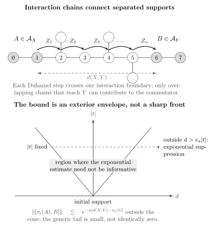
Only chains of overlapping interaction supports that connect $X$ to $Y$ enter the commutator recursion. Summability turns their path sum into an exponential exterior envelope. The shaded region is not a prediction of a sharp front, and the generic bound permits nonzero tails outside it.

Restoring units replaces every $\|\Phi\||t|$ in an exponent by $\|\Phi\||t|/\hbar$. In particular,

$$v_a = \frac{2C_{F_a}\|\Phi\|_{F_a}}{a\hbar}.$$

If graph distance is measured in lattice spacings, $a$ has units of inverse lattice spacing and $v_a$ has units of lattice spacings per unit time. The number $v_a$ changes with $a$, the chosen decay representation, and norm estimates. It is an upper-bound parameter, not a unique material constant.

Why the proof produces an exponential

The proof is a controlled version of the nested-commutator intuition. Fix $B\in\mathcal A_Y$ and define, for finite $X\subset\Lambda$,

$$C_B(X,t) = \sup_{A\in\mathcal A_X\setminus\{0\}} \frac{\|[\tau_t^\Lambda(A),B]\|}{\|A\|}.$$

Let $S_\Lambda(X)$ denote the interaction supports $Z\subset\Lambda$ that meet both $X$ and $\Lambda\setminus X$. Comparing the full evolution with the evolution generated only by terms internal to $X$, a Duhamel identity gives

$$\begin{aligned} C_B(X,t) &\leq 2\|B\|\mathbf 1_{X\cap Y\ne\varnothing}\\ &\quad+ 2\sum_{Z\in S_\Lambda(X)} \int_0^{|t|} \|\Phi(Z)\|C_B(Z,s)\,ds. \end{aligned}$$

The first term is the trivial commutator estimate when the supports already overlap. The integral term says that growth can leave $X$ only through an interaction term crossing its boundary.

Iterate the inequality. A nonzero $n$th-order contribution is indexed by a chain $Z_1,\ldots,Z_n$ of overlapping interaction supports: $Z_1$ crosses the boundary of $X$, each $Z_{j+1}$ overlaps $Z_j$, and the final set meets $Y$. The ordered time integral is the simplex volume

$$\int_{0\leq s_n\leq\cdots\leq s_1\leq |t|} ds_1\cdots ds_n = \frac{|t|^n}{n!}.$$

The interaction-norm estimate replaces every step by $\|\Phi\|_{F_a}$. Repeated use of the convolution inequality replaces the sum over intermediate sites by

$$C_{F_a}^{n-1}F_a(d(x,y)).$$

The remaining series is therefore proportional to

$$\sum_{n=1}^{\infty} \frac{(2C_{F_a}\|\Phi\|_{F_a}|t|)^n}{n!} = e^{2C_{F_a}\|\Phi\|_{F_a}|t|}-1.$$

Finally, the factor $e^{-a d(X,Y)}$ inside $F_a$ combines with the time exponential to give $e^{-a[d(X,Y)-v_a|t|]}$. The proof explains both the cone and its limitations: it overcounts possible paths and discards cancellations, so the velocity can be very nonsharp.

A nearest-neighbor chain audit

Consider a finite interval $\Lambda\subset\mathbb Z$ containing sites $0$ and $r>0$, with nearest-neighbor Hamiltonian

$$H_\Lambda = \sum_{j:\{j,j+1\}\subset\Lambda} h_{j,j+1}, \qquad \|h_{j,j+1}\|\leq J,$$

and let $A_0$ and $B_r$ be supported at sites $0$ and $r$. Expanding the finite-volume Heisenberg observable in operator norm,

$$\tau_t^\Lambda(A_0) = \sum_{n=0}^{\infty} \frac{(it/\hbar)^n}{n!} \operatorname{ad}_{H_\Lambda}^n(A_0),$$

where $\operatorname{ad}_{H_\Lambda}(A)=[H_\Lambda,A]$. Each commutator with a nearest-neighbor bond can enlarge the support by at most one site. Consequently,

$$[\operatorname{ad}_{H_\Lambda}^n(A_0),B_r]=0 \qquad \text{for }n<r.$$

This gives the correct microscopic picture: an operator path needs at least $r$ local steps to reach site $r$. It does not by itself prove a volume-uniform bound; that requires controlling the norms and number of every allowed path, which is the role of the $F$-function argument.

Reading a tolerance contour

Suppose an application has reduced the bound to

$$\|[\tau_t(A),B]\| \leq K e^{-a(r-v|t|)}.$$

To demand an error at most $\varepsilon<K$, it is sufficient that

$$r \geq v|t| + \frac{1}{a} \log\frac{K}{\varepsilon}.$$

For example, take $K=4$, $a=0.5$ per site, $r=40$ sites, $v=3$ sites per unit time, and $\varepsilon=10^{-4}$. The sufficient time window is

$$|t| \leq \frac{40-2\log(4\times10^4)}{3} \approx 6.27.$$

This is a certified exterior region for the chosen estimate, not a prediction that a physical front arrives at $t=40/3$.

Infinite-volume dynamics and unbounded on-site terms

Let $\Lambda_n\uparrow\Gamma$ be an increasing exhaustive sequence. Because the finite-volume estimate is uniform in $\Lambda_n$, a Duhamel comparison of two volumes shows that, for every local bounded $A$,

$$\tau_t(A) = \lim_{n\to\infty} \tau_t^{\Lambda_n}(A)$$

exists in operator norm, locally uniformly in $t$. The limit is independent of the exhaustion and extends to a strongly continuous one-parameter group of $*$-automorphisms of the quasi-local $C^*$-algebra. The same Lieb–Robinson estimate passes to the limit. This is a consequence of the decay hypotheses, not an automatic property of every formal infinite sum of Hamiltonian terms.

Arbitrary self-adjoint on-site Hamiltonians may also be allowed:

$$H_\Lambda = \sum_{x\in\Lambda}H_x + \sum_{Z\subset\Lambda}\Phi(Z),$$

even when the $H_x$ are unbounded, provided the intersite interaction terms $\Phi(Z)$ remain bounded and satisfy the decay norm. The on-site dynamics preserves support and operator norm, so an interaction-picture argument gives the same commutator estimate for bounded observables. Strong-operator topology enters the construction when unbounded generators are present; one must not silently promote every continuity statement to operator-norm continuity.

Infinite-dimensional on-site Hilbert spaces are therefore not the obstruction. The crucial distinction is between unbounded on-site terms, which this interaction-picture extension can handle, and generic unbounded intersite interactions, which the stated operator-norm theorem does not cover.

Consequences, each with its extra hypotheses

Local approximation. For a finite-dimensional spin system, average $\tau_t(A_X)$ over all unitaries outside the $R$-neighborhood $X_R$. The result is supported in $X_R$, and the averaging error is bounded by commutators with exterior unitaries. The theorem therefore gives an error proportional to $e^{-a(R-v_a|t|)}$.

Remote response. A local perturbation can influence a distant bounded measurement only through a time integral of a commutator. The same exterior envelope bounds that response. This is an upper bound on influence, not a claim that any signal actually propagates at $v_a$.

Generation of correlations and entanglement. Starting from suitably uncorrelated states, Lieb–Robinson estimates bound how quickly distant correlations or entanglement can be generated. Pre-existing correlations are not bounded by a dynamical commutator alone.

Exponential clustering. A spectral gap plus the ground-state and locality hypotheses of an exponential-clustering theorem imply decay of connected ground-state correlations. The Lieb–Robinson bound is an ingredient; it does not supply the gap or the ground-state assumptions.

Gapped phases and spectral flow. Along a uniformly gapped path of local Hamiltonians, additional hypotheses permit construction of a quasi-local spectral flow. Stability and phase-equivalence conclusions belong to those theorems, not to the commutator estimate by itself.

Algorithms. Truncating dynamics to a growing neighborhood gives locality-aware error estimates for finite-time Hamiltonian simulation. The complexity conclusion still depends on the algorithm, geometry, requested accuracy, and access model.

Scope boundaries

Time-dependent interactions

For a strongly continuous time-dependent interaction $\Phi(r)$ whose weighted norm is integrable on every compact time interval, the corresponding nonautonomous propagator exists and the same Duhamel iteration works. Define

$$I_{t,s}^{(a)} = \frac{C_{F_a}}{\hbar} \int_{\min(s,t)}^{\max(s,t)} \|\Phi(r)\|_{F_a}\,\mathrm dr.$$

The exact time factor becomes $e^{2I_{t,s}^{(a)}}-1$. Thus a driven system has a time-integrated locality budget rather than one fixed velocity. A uniform bound on $\|\Phi(r)\|_{F_a}$ recovers a linear cone, but a detailed driving protocol can give a sharper contour.

Power-law interactions

Do not apply the exponential-cone formula unchanged to an interaction with algebraic tails. For pair terms behaving schematically as

$$\|h_{xy}\| \lesssim d(x,y)^{-\alpha}$$

in spatial dimension $D$, modern optimal bounds depend on both $\alpha$ and $D$. For the interaction class of Tran and collaborators and $\alpha>2D$, the signal time obeys schematically

$$t_{\mathrm{signal}}(r) \gtrsim r^{\min\{1,\alpha-2D\}}.$$

Thus $2D<\alpha<2D+1$ gives a polynomial, non-linear cone, whereas $\alpha>2D+1$ permits a linear cone with algebraic rather than exponential leakage. Endpoint cases can have logarithmic qualifications. Every long-range claim must name the interaction class, norm, dimension, and transfer task.

Unbounded interactions and fermions

Harmonic and selected anharmonic oscillator lattices admit specialized bounds for bounded Weyl observables. Position and momentum themselves are unbounded, so their operator norms cannot be inserted into the theorem on this page. Generic unbounded intersite interactions require additional occupation, energy, or state-dependent control.

For CAR fermion systems, odd observables in disjoint regions anticommute rather than commute. Fermionic versions use even observables or graded commutators and a CAR-specific localization argument. The bosonic/spin tensor-product statement above must not be transferred word for word.

What the theorem does not establish

• It is not exact relativistic microcausality; the generic exterior tail is nonzero.
• It does not identify $v_a$ with a quasiparticle group velocity, butterfly velocity, entanglement velocity, transport velocity, or measured front.
• It does not say that correlations vanish outside the cone. With $H=0$, two distant spins may remain Bell-correlated while every relevant dynamical commutator is zero.
• It supplies no lower bound on propagation and does not establish ballistic transport.
• It does not imply a spectral gap, exponential clustering, an area law, or phase stability without additional hypotheses.
• It gives little information inside the cone and need not be numerically sharp.
• It is not automatically a theorem for continuum particles or relativistic quantum fields.
• It does not control generic unbounded observables or unbounded intersite interactions.

Common pitfalls

Writing only $Ce^{-\mu(d-vt)}$. The symbols conceal the metric, interaction class, support prefactor, norm, and volume uniformity. A valid application must expose those contracts.

Dropping the minus one in the exact bound. For disjoint supports the exact $F$-function estimate contains $e^{2C\|\Phi\||t|}-1$ and vanishes at $t=0$. The simpler cone envelope need not retain that sharp initial-time behavior.

Using the wrong sign. Exterior decay is $e^{-a[d-v|t|]}=e^{a(v|t|-d)}$. Reversing this sign predicts growth with distance.

Calling the velocity physical. A Lieb–Robinson velocity is convention- and estimate-dependent and is often much larger than a measured propagation speed.

Confusing commutators with correlations. A small commutator controls dynamically generated influence. It does not erase correlations already present in the state.

Treating all infinite-dimensional systems alike. Infinite-dimensional on-site spaces with bounded interactions fit the theorem. Generic unbounded intersite couplings do not.

Exercises

1. Disjoint local algebras

Embed $A\in\mathcal A_X$ and $B\in\mathcal A_Y$ into $\mathcal A_{X\cup Y}$ for $X\cap Y=\varnothing$ and prove $[A,B]=0$.

Solution

With the tensor factors ordered as $X$ followed by $Y$,

$$A=A_X\otimes I_Y, \qquad B=I_X\otimes B_Y.$$

Hence

$$AB=A_X\otimes B_Y=BA.$$

Embedding both operators into any larger local algebra merely adds further identity factors and does not change the conclusion.

2. A summable decay function on a lattice

For $p>\nu$, show that $F(r)=(1+r)^{-p}$ is uniformly summable on $\mathbb Z^\nu$ and outline why it obeys a convolution bound.

Solution

The number of lattice sites in a shell of radius $n$ grows as $O(n^{\nu-1})$. Therefore

$$\sum_{y\in\mathbb Z^\nu}F(d(x,y)) \lesssim 1+ \sum_{n=1}^{\infty} \frac{n^{\nu-1}}{(1+n)^p},$$

which converges because $p>\nu$, uniformly in $x$ by translation invariance.

For each intermediate site $z$, the triangle inequality implies that at least one of $d(x,z)$ and $d(z,y)$ is at least $d(x,y)/2$. Split the $z$ sum into those two cases. In either part, one factor is bounded by a constant times $F(d(x,y))$ and the other is summable. This gives

$$\sum_zF(d(x,z))F(d(z,y)) \leq C_FF(d(x,y))$$

with a finite constant independent of $x,y$.

3. Derive the cone form

Starting from the exact $F_a$ estimate, derive the exponential cone and the formula for $v_a$.

Solution

Use

$$\sum_{x\in X,y\in Y}F_a(d(x,y)) \leq \|F\|\min\{|X|,|Y|\}e^{-ad(X,Y)}$$

and $e^u-1\leq e^u$. The spatial and temporal exponentials combine as

$$e^{-ad(X,Y)} e^{2C_{F_a}\|\Phi\|_{F_a}|t|} = e^{-a[d(X,Y)-v_a|t|]},$$

where

$$v_a = \frac{2C_{F_a}\|\Phi\|_{F_a}}{a}$$

in units $\hbar=1$. Restoring units divides the right side by $\hbar$.

4. Minimum perturbative order

For a finite nearest-neighbor chain containing sites $0$ and $r>0$, prove that the norm-convergent Taylor series for $[\tau_t(A_0),B_r]$ has no nonzero term below order $r$.

Solution

The zeroth-order operator is supported at site $0$. Each commutator with the nearest-neighbor Hamiltonian can enlarge a support by at most one graph edge. Induction therefore gives

$$\operatorname{supp}(\operatorname{ad}_H^n(A_0)) \subseteq B_n(0) = \{j:d(j,0)\leq n\}.$$

Because $d(0,r)=r$, this support is disjoint from that of $B_r$ for $n<r$, so the corresponding commutator vanishes. On a two-sided chain, $B_n(0)=\{-n,\ldots,n\}$; growth to the left does not change the conclusion.

5. The ordered-time factorial

Show that the $n$-fold ordered integral in the Duhamel iteration equals $|t|^n/n!$ and explain its role in the bound.

Solution

The cube $[0,|t|]^n$ is partitioned, up to measure-zero boundaries, into $n!$ regions corresponding to the $n!$ possible orderings of its coordinates. All have the same volume, so the region $0\leq s_n\leq\cdots\leq s_1\leq|t|$ has volume $|t|^n/n!$.

After the path sums are bounded by powers of $2C_{F_a}\|\Phi\|_{F_a}$, these factorials turn the perturbation series into an exponential rather than a geometric series with a finite radius of convergence.

6. Correlations are not commutators

Place two distant qubits in $|\Phi^+\rangle=(|00\rangle+|11\rangle)/\sqrt2$ and take $H=0$. Compare the connected $z$ correlation with $[\sigma_z^{(1)}(t),\sigma_z^{(2)}]$.

Solution

In $|\Phi^+\rangle$,

$$\langle\sigma_z^{(1)}\sigma_z^{(2)}\rangle=1, \qquad \langle\sigma_z^{(1)}\rangle = \langle\sigma_z^{(2)}\rangle =0.$$

The connected correlation is therefore $1$. But $H=0$ makes every Heisenberg operator time independent, and the two Pauli operators act on distinct tensor factors, so

$$[\sigma_z^{(1)}(t),\sigma_z^{(2)}]=0.$$

The example separates pre-existing state correlation from dynamically generated influence.

7. Long-range regimes

Starting from $t_{\mathrm{signal}}(r)\gtrsim r^{\min\{1,\alpha-2D\}}$, classify the regimes $2D<\alpha<2D+1$ and $\alpha>2D+1$.

Solution

If $2D<\alpha<2D+1$, the exponent $\alpha-2D$ lies strictly between $0$ and $1$. Inverting the relation gives

$$r(t) \lesssim t^{1/(\alpha-2D)},$$

a polynomial cone wider than a linear one. If $\alpha>2D+1$, the minimum is $1$, so $r(t)\lesssim t$ and a linear cone is available. This schematic classification does not settle the threshold equalities, where logarithmic factors may occur.

8. Why oscillator bounds use Weyl operators

Explain why $q_x$ and $p_x$ cannot be inserted into this operator-norm theorem, whereas $W(f)=e^{i\phi(f)}$ can be used in a specialized oscillator bound.

Solution

The canonical position and momentum operators are unbounded, so $\|q_x\|=\|p_x\|=\infty$. An estimate proportional to those norms is vacuous. The Weyl operator $W(f)$ is unitary and therefore bounded with $\|W(f)\|=1$. Specialized oscillator theorems can consequently control commutators of Weyl operators even though the underlying fields are unbounded.

References

• S. Bachmann, S. Michalakis, B. Nachtergaele, and R. Sims, “Automorphic Equivalence within Gapped Phases of Quantum Lattice Systems,” Communications in Mathematical Physics 309, 835–871, 2012, doi:10.1007/s00220-011-1380-0.
• S. Bravyi, M. B. Hastings, and F. Verstraete, “Lieb–Robinson Bounds and the Generation of Correlations and Topological Quantum Order,” Physical Review Letters 97, 050401, 2006, doi:10.1103/PhysRevLett.97.050401.
• M. B. Hastings and T. Koma, “Spectral Gap and Exponential Decay of Correlations,” Communications in Mathematical Physics 265, 781–804, 2006, doi:10.1007/s00220-006-0030-4.
• T. Kuwahara and K. Saito, “Strictly Linear Light Cones in Long-Range Interacting Systems of Arbitrary Dimensions,” Physical Review X 10, 031010, 2020, doi:10.1103/PhysRevX.10.031010.
• E. H. Lieb and D. W. Robinson, “The Finite Group Velocity of Quantum Spin Systems,” Communications in Mathematical Physics 28, 251–257, 1972, doi:10.1007/BF01645779.
• B. Nachtergaele, H. Raz, B. Schlein, and R. Sims, “Lieb–Robinson Bounds for Harmonic and Anharmonic Lattice Systems,” Communications in Mathematical Physics 286, 1073–1098, 2009, doi:10.1007/s00220-008-0630-2.
• B. Nachtergaele and R. Sims, “Lieb–Robinson Bounds and the Exponential Clustering Theorem,” Communications in Mathematical Physics 265, 119–130, 2006, doi:10.1007/s00220-006-1556-1.
• B. Nachtergaele and R. Sims, “Lieb–Robinson Bounds in Quantum Many-Body Physics,” Contemporary Mathematics 529, 141–176, 2010, doi:10.1090/conm/529/10429.
• B. Nachtergaele, R. Sims, and A. Young, “Lieb–Robinson Bounds, the Spectral Flow, and Stability of the Spectral Gap for Lattice Fermion Systems,” Contemporary Mathematics 717, 93–115, 2018, doi:10.1090/conm/717/14443.
• B. Nachtergaele, R. Sims, and A. Young, “Quasi-Locality Bounds for Quantum Lattice Systems. Part I. Lieb–Robinson Bounds, Quasi-Local Maps, and Spectral Flow Automorphisms,” Journal of Mathematical Physics 60, 061101, 2019, doi:10.1063/1.5095769.
• M. C. Tran, A. Y. Guo, C. L. Baldwin, A. Ehrenberg, A. V. Gorshkov, and A. Lucas, “The Lieb–Robinson Light Cone for Power-Law Interactions,” Physical Review Letters 127, 160401, 2021, doi:10.1103/PhysRevLett.127.160401.