From Spectra to Atomic Physics

Atomic physics grew from a very concrete puzzle: atoms emit and absorb light at sharply defined frequencies. Long before there was a Schrödinger equation, spectroscopy showed that atoms have reproducible internal structure. The modern theory explains those regularities with Hamiltonians, energy eigenstates, angular momentum, transition amplitudes, and controlled approximations.

This page is a bridge. It does not replace the canonical Hydrogen Atom calculation, the historical Line Spectra page, or the compact Hydrogen Spectrum Formula reference. Its purpose is to show how the pieces fit together.

Energy Differences

The most important conceptual move is to read spectral frequencies as energy differences. If an atom emits light of frequency $\nu$, the photon carries energy

$$E_\gamma=h\nu.$$

Modern quantum mechanics describes the emitting atom as moving from a higher-energy state to a lower-energy state:

$$h\nu = E_i-E_f.$$

Absorption reverses the process. Light of the appropriate frequency can drive a transition from $E_f$ to $E_i$, subject to the relevant selection rules and matrix elements.

This is more than a formula. It changes the object of explanation. A classical orbit picture tries to relate radiation to the mechanical frequency of a charge in motion. Atomic spectra instead force attention onto differences between allowed stationary energies. The Rydberg Formula made this difference structure visible before the modern state-vector language existed.

For hydrogen, the empirical pattern can be written as

$$\frac{1}{\lambda} = R_H \left( \frac{1}{n_f^2} - \frac{1}{n_i^2} \right), \qquad n_i>n_f.$$

Since $\nu=c/\lambda$, this suggests a family of energies proportional to $-1/n^2$:

$$E_n = -hc\frac{R_H}{n^2}.$$

The minus sign matters. The bound states lie below the ionization threshold, conventionally placed at $E=0$. Lines arise when the atom moves between bound states, or between a bound state and the continuum.

Bohr as a Stepping Stone

Bohr’s model joined Rutherford’s nuclear atom, Planck’s constant, and the spectral difference law. It used stationary orbits, quantized angular momentum, and the frequency condition

$$h\nu=E_i-E_f.$$

For hydrogen, it produced

$$E_n \approx -\frac{13.6\,\mathrm{eV}}{n^2}, \qquad n=1,2,3,\ldots,$$

and therefore reproduced the leading Rydberg pattern. That success was real. It explained why hydrogen line positions organize into series and why atomic stability required something beyond naive classical electrodynamics.

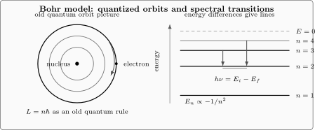
The Bohr model was a historically essential bridge from spectral regularities to energy levels. Modern atomic physics keeps the energy-level and transition-frequency ideas but replaces literal orbits with wavefunctions, angular-momentum eigenstates, and transition amplitudes.

The model is not modern quantum mechanics. It does not provide a Hilbert-space state, a systematic operator theory, general transition probabilities, spin, many-electron structure, or a controlled treatment of measurement. Its value is that it identified the right spectral scale and the right organizing principle: atomic radiation is governed by level differences.

The historical details belong to Bohr Model and Sommerfeld Model. The limits of the old framework are collected in Limits of Old Quantum Theory.

Wave-Mechanical Hydrogen

Wave mechanics keeps the Coulomb attraction but changes the mathematical problem. Instead of selecting allowed orbits by hand, one solves the stationary Schrödinger equation for the relative electron-proton coordinate:

$$\hat H\psi(\mathbf r) = E\psi(\mathbf r),$$

with

$$\hat H = -\frac{\hbar^2}{2\mu}\nabla^2 - \frac{e^2}{4\pi\epsilon_0r}.$$

Here $\mu$ is the reduced mass. The allowed bound states are normalizable eigenfunctions. In spherical coordinates they separate as

$$\psi_{n\ell m}(r,\theta,\phi) = R_{n\ell}(r)Y_\ell^m(\theta,\phi).$$

The quantum numbers have distinct meanings:

• $n$ labels the principal energy scale in the ideal Coulomb problem;
• $\ell$ labels orbital angular momentum;
• $m$ labels the projection of orbital angular momentum on a chosen axis.

The leading nonrelativistic energies are

$$E_n = -\frac{\mu e^4}{2(4\pi\epsilon_0)^2\hbar^2} \frac{1}{n^2}.$$

This result explains why the old Rydberg pattern worked for hydrogen while replacing the orbit picture with wavefunctions and boundary conditions. The canonical derivation, radial equations, degeneracy counting, and orbital interpretation belong to Hydrogen Atom, Radial Wavefunctions, Atomic Orbitals, and Degeneracy of the Hydrogen Atom.

Selection Rules and Spectroscopy

Energy differences locate possible spectral lines. They do not by themselves determine which lines are bright, weak, or absent. A transition probability also depends on how the atom couples to the radiation field.

In the electric-dipole approximation, a typical transition amplitude contains a matrix element of the position operator:

$$\mathbf d_{fi} = -e \langle f|\mathbf r|i\rangle.$$

If this matrix element vanishes by symmetry, the electric-dipole transition is forbidden at that order. For hydrogenic orbital states, the familiar electric-dipole selection rules include

$$\Delta\ell=\pm1, \qquad \Delta m=0,\pm1,$$

with polarization determining which $\Delta m$ channels are driven. The symmetry derivation is developed in Dipole Transitions. More refined spectroscopy adds spin, fine structure, hyperfine structure, external fields, line broadening, and higher multipoles.

This is where atomic physics becomes a precision discipline. The theory of line positions uses Hamiltonian eigenvalues. The theory of line strengths uses transition matrix elements. The theory of measured line shapes uses lifetimes, thermal motion, collisions, instrumental resolution, and environmental perturbations. See Selection Rules, Applications to Atomic Spectra, Selection Rules and Transition Rates, and Spectroscopy.

AMO Path

Modern atomic, molecular, and optical physics extends the spectral lesson in several directions.

First, atoms become controlled quantum systems. Lasers as Quantum Technology provide narrowband fields that drive selected transitions, cool atoms, trap particles, and measure small shifts. Magnetic Resonance shows the same transition logic in spin systems.

Second, hydrogen becomes the template rather than the endpoint. Hydrogenic ions preserve the one-electron Coulomb structure with nuclear charge $Z$, while multi-electron atoms require electron-electron interactions, antisymmetry, spin–orbit effects, and approximation methods. The simple $-1/n^2$ spectrum is a starting benchmark, not a universal law.

Third, precision corrections become physically meaningful. Fine structure, Lamb shifts, hyperfine splitting, Zeeman shifts, Stark shifts, and finite-nuclear-size effects are not decorations added after the real theory. They are part of how experiments test Hamiltonians, symmetries, quantum electrodynamics, and constants.

Fourth, spectroscopy links bound-state physics to scattering and the continuum. Ionization thresholds, photoabsorption, Rydberg states, resonances, and continuum wavefunctions connect atomic spectra to collision theory and field quantization.

The practical reading path is:

• start with Line Spectra and Rydberg Formula;
• use Bohr Model as the old-quantum-theory bridge;
• move to Coulomb Potential and Hydrogen Atom;
• add Spherical Harmonics and Angular Momentum Algebra;
• then study transition rates, selection rules, perturbations, and experimental spectroscopy.

Common Mistakes

• Treating spectral line positions as if they also determined line intensities.
• Reading Bohr orbits as literal modern electron trajectories.
• Forgetting that the Rydberg formula is a leading hydrogenic result, not a complete theory of all atoms.
• Saying that spectroscopy proves every quantum spectrum is discrete. Bound atomic states are discrete, while continua and scattering states also exist.
• Ignoring reduced mass when comparing high-precision hydrogen numbers.
• Mixing historical explanation with canonical derivation. The history motivates the problem; the Schrödinger eigenvalue problem solves the leading hydrogen model.

Cross-Links

• Atomic Structure and Spectra
• Line Spectra
• Balmer Formula
• Rydberg Formula
• Bohr Model
• Hydrogen Atom
• Hydrogen Spectrum Formula
• Atomic Orbitals
• Selection Rules and Transition Rates
• Selection Rules
• Applications to Atomic Spectra
• Dipole Transitions
• Spectroscopy

References

• J. J. Balmer, “Notiz ueber die Spectrallinien des Wasserstoffs,” Annalen der Physik und Chemie 25, 80-87 (1885).
• J. R. Rydberg, “Recherches sur la constitution des spectres d’emission des elements chimiques,” Kungliga Svenska Vetenskapsakademiens Handlingar 23, 1-177 (1890).
• N. Bohr, “On the Constitution of Atoms and Molecules,” Philosophical Magazine 26, 1-25 (1913), DOI: 10.1080/14786441308634955.
• E. Schrödinger, “Quantisierung als Eigenwertproblem,” Annalen der Physik 79, 361-376 (1926), DOI: 10.1002/andp.19263840404.
• G. Herzberg, Atomic Spectra and Atomic Structure, Dover, 1944.
• B. H. Bransden and C. J. Joachain, Physics of Atoms and Molecules, 2nd ed., Pearson, 2003.
• W. Demtröder, Atoms, Molecules and Photons, 2nd ed., Springer, 2010.
• H. Haken and H. C. Wolf, The Physics of Atoms and Quanta, 7th ed., Springer, 2005.

Exercises

1. Explain why the Rydberg formula suggests energy differences rather than a list of unrelated wavelengths.

Solution

The formula writes spectral wavenumbers as differences of terms proportional to $1/n^2$. Since photon energy is $hc/\lambda$, the same structure is naturally read as $E_i-E_f$. This does not by itself derive the atomic Hamiltonian, but it strongly suggests that atoms have a set of stationary energies and that spectral lines compare pairs of them.

2. In what sense did the Bohr model succeed, and in what sense was it superseded?

Solution

It succeeded by reproducing the leading hydrogen energy scale and the Rydberg spectral pattern while introducing stationary states and transition frequencies. It was superseded because its orbit picture and quantization rules are not a systematic quantum theory. Wave mechanics replaces selected orbits with wavefunctions, operators, boundary conditions, and probability amplitudes.

3. Why do energy eigenvalues alone not determine a complete spectrum observed in a laboratory?

Solution

Energy differences determine candidate transition frequencies. The observed spectrum also depends on transition matrix elements, selection rules, polarization, state preparation, line broadening, external fields, finite lifetime, collisions, thermal motion, and detector resolution. A complete spectroscopy calculation therefore needs both the Hamiltonian spectrum and the dynamics of coupling to light or other probes.