Canonical Plots Gallery

Canonical wave-mechanics systems are often recognized by their plots before they are recognized by their formulas. Hard-wall nodes, evanescent tails, tunneling suppression, Gaussian spreading, oscillator ladders, angular lobes, and Landau-level degeneracy each have a characteristic visual signature.

The gallery below is a visual index, not a replacement for the linked derivations. The panels are schematic and dimensionless: amplitudes are rescaled, offsets are chosen for readability, and only the qualitative structure is meant to be compared across models.

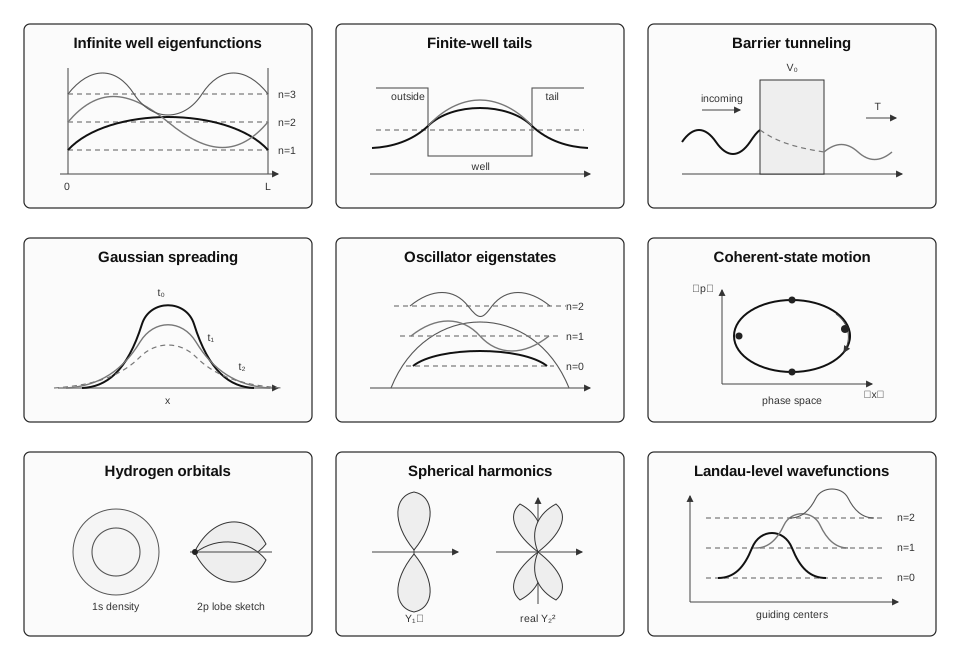
A compact visual index for standard wave-mechanics models. The panels show square-well eigenfunctions, finite-well tails, barrier tunneling, Gaussian spreading, harmonic-oscillator eigenstates, coherent-state motion, hydrogen orbital shapes, spherical-harmonic angular structure, and Landau-level wavefunctions. All scales are schematic.

How to Use the Gallery

Use this page as a recognition aid. When a calculation produces a wavefunction, density, spectrum, or numerical plot, compare it with the relevant panel and then follow the linked canonical page for the actual assumptions and normalization conventions.

A good plot should make three things visible:

• the physical setup, such as walls, barriers, wells, angular constraints, or magnetic field;
• the boundary or asymptotic behavior, such as nodes, continuity, decay, or oscillatory scattering tails;
• the scale or quantum number being varied, such as $n$, $L$, $\omega$, $\ell_B$, or time.

Plot Index

Panel	What to Look For	Main Lesson	Canonical Page
Infinite well eigenfunctions	Nodes at hard walls and increasing oscillation count with $n$	Boundary conditions quantize energy	Infinite Square Well
Finite-well tails	Oscillatory interior with exponential decay outside the well	Finite barriers do not force $\psi$ to vanish	Finite Square Well
Barrier tunneling	Evanescent behavior inside the barrier and smaller transmitted wave	Transmission is a current ratio, not just an amplitude sketch	Rectangular Barrier Tunneling
Gaussian spreading	A localized packet broadens as time increases	Free-particle dispersion changes width while preserving norm	Wave Packet Spreading
Oscillator eigenstates	Parabolic potential, equally spaced levels, alternating parity	Quadratic potentials produce a universal ladder	Quantum Harmonic Oscillator
Coherent-state motion	Phase-space orbit of the packet center	Coherent states preserve their Gaussian shape in a harmonic potential	Coherent States
Hydrogen orbitals	Radial localization and angular lobes	Central potentials separate into radial and angular structure	Hydrogen Atom
Spherical harmonics	Angular lobes and nodal surfaces	Angular wavefunctions are geometry, not radial dynamics	Spherical Harmonics
Landau-level wavefunctions	Oscillator-like transverse states at different guiding centers	Uniform magnetic fields quantize cyclotron motion and create degeneracy	Landau Levels

Standards for Future Plots

Future model pages should use the same visual discipline:

• label axes or state when axes are schematic;
• show potentials and wavefunctions on separate vertical scales when necessary;
• distinguish $\psi$ from $\lvert\psi\rvert^2$;
• state whether states are square-normalized, box-normalized, delta-normalized, or flux-normalized;
• mark classical turning points, walls, interfaces, and asymptotic regions when they matter;
• avoid comparing amplitudes across different panels unless a shared normalization is stated.

For generated plots, the accompanying notebook or source should record the dimensionless variables, parameter values, and validation check. A plot of a finite-difference eigenfunction, for example, should report the grid spacing and compare the numerical energy with the analytic or benchmark value.

Common Mistakes

• Treating schematic vertical offsets as physical energy values.
• Comparing unnormalized wavefunction heights between different systems.
• Plotting $\psi$ when the physical question is about $\lvert\psi\rvert^2$.
• Hiding boundary behavior by cropping the plot too tightly.
• Drawing tunneling as a literal classical path through a wall rather than an evanescent wave.
• Showing hydrogen orbitals without saying whether the plot is an amplitude, probability density, or surface of constant probability density.
• Plotting gauge-dependent Landau wavefunctions without stating the gauge.

Where This Is Used

• Map of Canonical Systems gives the conceptual index that this page visualizes.
• Visualization Gallery records figure sources, validation status, and notebook-export standards for visual assets.
• Common Hamiltonians gives the matching Hamiltonian lookup table.
• Spectra and Eigenfunctions Table supplies the formulas behind many panels.
• Boundary Conditions Table explains the endpoint and matching behavior visible in the one-dimensional panels.
• Limiting Cases Table explains how the same models simplify in transparent, opaque, classical, and continuum limits.
• Dimensionless Parameters Table names the scale-free parameters that should be stated on quantitative plots.
• Normalization Table helps decide whether a plotted curve is an amplitude, density, radial density, or flux-normalized mode.
• Normalization Conventions explains why plotted wavefunctions may use different normalization conventions.

References

• D. J. Griffiths and D. F. Schroeter, Introduction to Quantum Mechanics, 3rd ed., Cambridge University Press, 2018.
• R. Shankar, Principles of Quantum Mechanics, 2nd ed., Springer, 1994.
• C. Cohen-Tannoudji, B. Diu, and F. Laloë, Quantum Mechanics, Wiley, 1977.
• L. D. Landau and E. M. Lifshitz, Quantum Mechanics: Non-Relativistic Theory, 3rd ed., Pergamon, 1977.

Exercises

1. In the finite-well panel, why do the tails outside the well matter physically even though the particle is classically forbidden there?

Solution

The finite outside region is not excluded from the Hilbert space. For a bound state below the outside potential, the solution outside the well is evanescent rather than zero. These tails affect normalization, matching conditions, bound-state energies, tunneling intuition, and overlap with nearby wells.

2. A numerical plot of a Landau-gauge wavefunction shows a Gaussian-like oscillator state centered at a value $x_0$. What should be checked before calling it a physical density plot?

Solution

One should state the gauge, the magnetic length $\ell_B$, the relation between $x_0$ and the conserved momentum, and the normalization convention. The wavefunction shape is gauge dependent, while the Landau-level energy and degeneracy per area are gauge-invariant physical statements.