Visualization Gallery

Visualizations are part of the evidence layer of a wave-mechanics reference. A good figure shows the physical setup, the mathematical object being plotted, the scale choices, and the check that makes the plot trustworthy. A decorative plot without a stated convention can be worse than no plot, because it invites readers to compare amplitudes, densities, or gauges incorrectly.

This gallery records visualization assets for the Wave Mechanics and Model Systems volume and sets the standard for adding more. The conceptual visual index is Canonical Plots Gallery; this page focuses on asset provenance, notebook sources, captions, accessibility, and validation.

Current Static Gallery

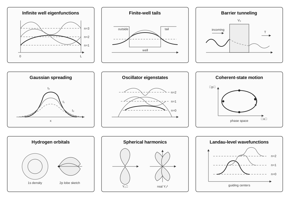
The current static overview asset for canonical wave mechanics. It is a schematic nine-panel SVG generated from a tracked TikZ source, not a numerical notebook output. The panels are intended for recognition: square-well nodes, finite-well tails, barrier tunneling, Gaussian spreading, oscillator states, coherent motion, hydrogenic structure, spherical harmonics, and Landau-gauge wavefunctions.

Asset	Source	Validation Status	Canonical Page
/figures/wave-mechanics/canonical-plots-gallery.svg	/figures-src/wave-mechanics/canonical-plots-gallery.tex	committed static SVG; XML parsed and full site build passes	Canonical Plots Gallery

This is the only committed static gallery asset in this volume as of July 14, 2026. Notebook-generated figures should be added only after their source notebook includes a numerical validation cell and the exported figure has an explanatory caption.

Admission Checklist

A visualization belongs in this gallery only when it has:

• a stable asset path under public/figures/wave-mechanics/;
• a source path, either TikZ under public/figures-src/wave-mechanics/ or a notebook under notebooks/wave-mechanics-canonical-systems/;
• alt text that states what the image shows, not merely the file name;
• a caption that names the plotted quantity, normalization convention, and parameter values;
• a validation statement, such as an analytic comparison, conservation check, convergence check, or explicit declaration that the figure is schematic;
• a link to the canonical page where the physics is explained.

Animated GIFs or videos should satisfy the same checklist and also state the time step, playback speed, and whether the animation is schematic or generated from a validated computation.

Candidate Notebook Visualizations

The first notebook batch is validation-first and NumPy-only. It deliberately does not commit static exported plots yet. The table below records the most useful visualizations to export once plotting support and captions are added.

Candidate Visualization	Notebook Source	What the Figure Should Show	Required Check Before Export
Infinite-well eigenfunctions and energy convergence	one-dimensional-bound-systems/infinite-square-well.ipynb	first few eigenfunctions with hard-wall nodes and a convergence table for $E_n$	eigenvalues approach $n^2\pi^2\hbar^2/(2mL^2)$ and eigenvectors are grid-orthonormal
Finite-well bound-state tails	one-dimensional-bound-systems/finite-square-well-bound-states.ipynb	interior oscillation, exterior evanescent decay, and depth-dependent bound-state count	bound-state count changes with depth and edge leakage is negligible
Gaussian packet spreading	free-motion/gaussian-wave-packet-spreading.ipynb	packet density at several times with envelope broadening	norm conservation and analytic width $\sigma_x(t)$
Barrier packet scattering	scattering-tunneling/barrier-scattering-wave-packet.ipynb	incident, reflected, transmitted, and barrier-neighborhood probability regions	final probability accounting and norm conservation
Oscillator eigenstates	harmonic-oscillator/harmonic-oscillator-eigenstates.ipynb	parabolic potential, first eigenstates, parity pattern, and energy ladder	energy errors and parity overlaps
Two-level dynamics	two-level-systems/two-level-system-dynamics.ipynb	transition probability versus time with analytic curve	agreement with the exact sinusoidal transition probability
Hydrogen radial functions	hydrogenic/hydrogen-radial-wavefunctions.ipynb	$r^2\lvert R_{n\ell}(r)\rvert^2$ for low states	radial normalization and most-probable-radius check
Real spherical harmonics	three-dimensional/spherical-harmonics-gallery.ipynb	angular lobes or signed angular functions	angular normalization and orthogonality
Landau-level oscillator states	electromagnetic-fields/landau-levels.ipynb	transverse oscillator states and guiding-center spacing	oscillator spectrum and finite-area degeneracy estimate

Candidates are not gallery entries until their exported assets exist. This distinction keeps the page useful without pretending a planned image is already part of the reference.

Caption Requirements

Every figure caption should answer five questions:

1. What is plotted: $\psi$, $\lvert\psi\rvert^2$, $r^2\lvert R\rvert^2$, energy, current, or probability?
2. What convention is used: square normalization, box normalization, flux normalization, grid normalization, or a schematic rescaling?
3. What parameters are fixed: $L$, $V_0$, $a$, $\omega$, $\ell_B$, $n$, $\ell$, $m$, or dimensionless combinations?
4. What is the physical lesson: boundary condition, tunneling, spreading, parity, degeneracy, or gauge dependence?
5. What check supports the figure: exact formula, limiting case, norm conservation, current conservation, or convergence?

If a figure cannot answer these questions in a compact caption, it needs a nearby explanatory paragraph before it belongs in the gallery.

Accessibility and Alt Text

Alt text should describe the visual content and the physics cue. For example, “Three Gaussian wave packets at later times, each broader and shifted right” is useful. “Gaussian plot” is not. For color-dependent plots, do not encode essential distinctions only by color; use labels, line styles, markers, or panel separation.

For dense mathematical visuals, the caption should carry the scientific meaning so that the figure is not the only source of information.

Common Mistakes

• Exporting a notebook plot before the notebook has validation cells.
• Plotting $\psi$ when the caption interprets $\lvert\psi\rvert^2$.
• Omitting grid spacing, box size, or boundary conditions from numerical figures.
• Showing a Landau-gauge wavefunction without saying the gauge.
• Cropping away tails, nodes, interfaces, or turning points that carry the physics.
• Using the same vertical scale for different quantities without saying so.
• Adding an animation without a time scale or normalization check.

Where This Is Used

• Canonical Plots Gallery is the canonical visual-recognition page for standard models.
• Numerical Notebooks Index lists the source notebooks that should eventually export validated figures.
• Benchmark Problems defines the checks required before notebook outputs become gallery assets.
• Problem-Solving Patterns explains the recurring physics that visuals should make visible.
• Normalization Table helps captions distinguish amplitude, density, radial density, and flux-normalized modes.

References

• D. J. Griffiths and D. F. Schroeter, Introduction to Quantum Mechanics, 3rd ed., Cambridge University Press, 2018.
• R. Shankar, Principles of Quantum Mechanics, 2nd ed., Springer, 1994.
• E. Tufte, The Visual Display of Quantitative Information, 2nd ed., Graphics Press, 2001.
• C. R. Harris et al., “Array programming with NumPy,” Nature 585, 357-362 (2020).

Exercises

1. A notebook exports a plot of a finite-well eigenfunction but does not state whether the curve is $\psi$ or $\lvert\psi\rvert^2$. Why should the plot stay out of the gallery?

Solution

The interpretation changes completely. $\psi$ can be signed or complex, while $\lvert\psi\rvert^2$ is a probability density. Without the plotted quantity and normalization convention, readers cannot compare amplitudes, tails, nodes, or probabilities correctly.

2. A Gaussian-packet animation conserves norm but disagrees with the analytic packet width. What should the caption or notebook explain before the animation is accepted?

Solution

It should explain whether the initial packet convention matches the analytic formula, whether finite-box effects or grid dispersion are visible, and whether the time step or propagation method introduces error. Norm conservation alone does not validate the width or phase evolution.