The Minimal Language of Quantum Mechanics

The minimal language of quantum mechanics is the small collection of mathematical objects and rules needed to turn a preparation procedure into probabilities for possible experimental outcomes. In its most portable form, the language consists of states, physical transformations, measurements, and composition rules.

This page is a one-pass map, not a substitute for the canonical derivations. It emphasizes the density-operator formulation because one formula then covers pure states, mixed preparations, subsystems of entangled systems, closed-system evolution, open-system processes, and generalized measurements. Readers meeting the formalism for the first time may replace density operators by kets and general measurements by projectors wherever the corresponding special case is stated.

The Core Dictionary

Physical task or idea	Mathematical object	Operational role
Preparation	state $\rho$	encodes probabilities for every allowed measurement
Pure preparation	ray $[	psi\rangle]$
Observable quantity	self-adjoint operator $A$	packages outcomes and projectors for an ideal sharp measurement
General measurement	effects $lbrace E_a\rbrace_a$	assigns a positive operator to each outcome $a$
Outcome probability	$p(a)=\operatorname{Tr}(\rho E_a)$	connects a state and a specified measurement
Conditional state change	quantum instrument $\lbrace\mathcal I_a\rbrace_a$	describes both the outcome and its state update
Closed-system evolution	unitary operator $U$	sends $\rho$ to $U\rho U^\dagger$
General physical process	quantum channel $\mathcal E$	sends input states to output states
Composite system	tensor product $\mathcal H_A\otimes\mathcal H_B$	allows joint, product, and entangled states
Subsystem state	partial trace	gives $\rho_A=\operatorname{Tr}_B\rho_{AB}$
Symmetry	unitary or antiunitary transformation	preserves transition probabilities and the relevant physical structure

The table separates three notions that are often conflated:

1. a state describes a preparation;
2. a measurement specifies which outcomes are being distinguished;
3. a dynamical map describes what happens between preparation and measurement.

No probability is determined until all three parts of the experimental contract are fixed.

The Preparation-to-Prediction Contract

Let a laboratory setting $\lambda$ prepare a state $\rho_\lambda$. Let the system undergo a physical process $\mathcal E$, and let the final measurement have effects $E_a$. The predicted outcome law is

$$p(a\mid\lambda) =\operatorname{Tr}\!\left[ E_a\,\mathcal E(\rho_\lambda) \right].$$

This compact expression is the operational backbone of the theory. It says what is prepared, what transformation is assumed, what is measured, and which probability is predicted. The ingredients must satisfy

$$\begin{aligned} &\rho_\lambda\ge 0, &&\operatorname{Tr}\rho_\lambda=1,\\ &E_a\ge 0, &&\sum_a E_a=I,\\ &\mathcal E\text{ is completely positive}, &&\operatorname{Tr}\mathcal E(\rho)=1 \quad\text{for a channel}. \end{aligned}$$

These conditions ensure that probabilities are nonnegative, normalized, and remain consistent when the system is entangled with an unobserved reference. The complete-positivity condition is developed in Completely Positive Maps.

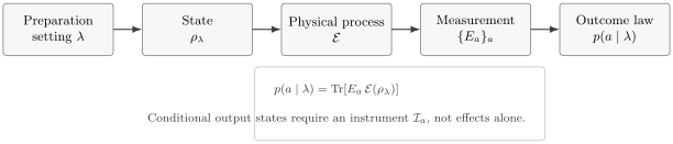
The minimal operational cycle. A model assigns a state $\rho_\lambda$ to a preparation, a channel $\mathcal E$ to the intervening process, and effects $E_a$ to the outcomes. The Born rule produces the probability law. Predicting post-measurement states requires an instrument $\mathcal I_a$, which contains more information than the effects alone.

Experiments return finite data rather than exact probabilities. If outcome $a$ occurs $n_a$ times in $N$ repeated trials, its empirical frequency is $f_a=n_a/N$. Statistical inference compares the frequency vector with the model probabilities while accounting for sampling error, drift, and model uncertainty. Quantum mechanics supplies $p(a\mid\lambda)$; it does not make a finite data set equal to that probability distribution.

States Describe Preparations

A quantum state is the object from which the theory predicts measurement statistics for a specified preparation. The most general state used here is a density operator

$$\rho\ge 0, \qquad \operatorname{Tr}\rho=1.$$

Positivity means $\langle\phi|\rho|\phi\rangle\ge 0$ for every ket $|\phi\rangle$. Together with unit trace, it guarantees that the probabilities computed from $\rho$ are nonnegative and normalized.

Pure states and rays

A pure state is an extremal state represented by a rank-one projector,

$$\rho_\psi=|\psi\rangle\langle\psi|, \qquad \langle\psi|\psi\rangle=1.$$

The kets $|\psi\rangle$ and $e^{i\chi}|\psi\rangle$ define the same projector and therefore the same physical pure state. The physical state is a ray, not one preferred vector on that ray. Relative phases between components of a state, however, can affect probabilities and are generally observable through interference.

Mixed states

A density operator can be written as an ensemble

$$\rho=\sum_j q_j|\psi_j\rangle\langle\psi_j|, \qquad q_j\ge 0, \qquad \sum_j q_j=1.$$

Such a decomposition can describe a preparation that randomly selects pure states. It is not unique: different ensembles can produce the same $\rho$ and hence the same statistics for every measurement on the system. The density operator, rather than a chosen ensemble decomposition, is the operational state. Density Operators develops this point and the purity criterion $\operatorname{Tr}(\rho^2)=1$.

A state is not yet a probability distribution

The same state gives different distributions for different measurements. For example, $|0\rangle$ predicts a certain outcome for a measurement in the $\{|0\rangle,|1\rangle\}$ basis but a uniform distribution for a measurement in the $\{|+\rangle,|-\rangle\}$ basis. Asking for “the probabilities in a state” is incomplete until the measurement is named.

The state also need not be interpreted as a list of hidden classical properties. It is, at minimum, the predictive object associated with a preparation. Interpretations may make additional claims about what the state represents, but the probability calculus does not require those claims here.

Measurements Connect States to Outcomes

A measurement is not specified by an outcome label alone. It requires a mathematical description of how each possible outcome couples to the state.

General outcome probabilities

A measurement with discrete outcomes $a$ is represented at the probability level by a positive-operator-valued measure, or POVM,

$$E_a\ge 0, \qquad \sum_a E_a=I.$$

The Born rule is

$$p(a\mid\rho)=\operatorname{Tr}(\rho E_a).$$

Normalization follows immediately:

$$\sum_a p(a\mid\rho) =\operatorname{Tr}\!\left(\rho\sum_a E_a\right) =\operatorname{Tr}\rho =1.$$

This formula covers ideal projective measurements, noisy detectors, coarse-grained readout, and measurements with more outcomes than the Hilbert space dimension. Generalized Measurements Overview explains how effects arise from measurement operators.

Sharp observables as a special case

For an ideal discrete observable, a self-adjoint operator has spectral form

$$A=\sum_a aP_a, \qquad P_aP_b=\delta_{ab}P_a, \qquad \sum_a P_a=I.$$

The outcome labels are the eigenvalues $a$, and the effects are the orthogonal projectors $E_a=P_a$. The expectation value is therefore

$$\langle A\rangle_\rho =\sum_a a\,p(a\mid\rho) =\operatorname{Tr}(\rho A).$$

An expectation value is an ensemble mean, not necessarily a possible outcome and not necessarily the most probable outcome.

Outcome probabilities do not determine state update

Effects determine probabilities, but not by themselves what state remains after an outcome. A quantum instrument assigns a completely positive map $\mathcal I_a$ to each outcome:

$$p(a\mid\rho)=\operatorname{Tr}[\mathcal I_a(\rho)], \qquad \rho_a =\frac{\mathcal I_a(\rho)}{p(a\mid\rho)}.$$

For an ideal projective measurement with the Lüders update,

$$\mathcal I_a(\rho)=P_a\rho P_a, \qquad \rho_a =\frac{P_a\rho P_a} {\operatorname{Tr}(\rho P_a)}.$$

Other instruments can have the same effects and therefore the same outcome probabilities while producing different conditional states. The State Update Rule owns the projective derivation; later open-systems pages treat instruments in full.

Dynamics Transform States

The dynamics specifies how a state changes between preparation and measurement. It must be distinguished from both the state and the measurement model.

Closed systems

An isolated system evolves unitarily. If $U(t,t_0)$ is the evolution operator,

$$\rho(t) =U(t,t_0)\rho(t_0)U^\dagger(t,t_0).$$

For a pure state this becomes

$$|\psi(t)\rangle =U(t,t_0)|\psi(t_0)\rangle.$$

With a time-independent self-adjoint Hamiltonian $H$,

$$U(t,t_0) =\exp\!\left[-\frac{i}{\hbar}H(t-t_0)\right],$$

and the state satisfies the Schrödinger equation. Unitarity preserves inner products, trace, positivity, and the spectrum of $\rho$. The derivation and the time-dependent case belong to Unitary Time Evolution and Time-Dependent Hamiltonians.

Open systems and laboratory processes

A system interacting with an environment, undergoing noise, or passing through a general control sequence is described by a quantum channel $\mathcal E$ at the input-output level:

$$\rho_{\mathrm{out}}=\mathcal E(\rho_{\mathrm{in}}).$$

A channel is linear, completely positive, and trace preserving. Every unitary evolution defines a channel, but most channels are not unitary on the system alone. This broader language is essential for decoherence, measurement, feedback, and quantum information processing. The canonical treatment begins with Quantum Operations.

Pictures move the time dependence

The Schrödinger picture places time dependence in states. The Heisenberg picture instead evolves observables,

$$A_H(t)=U^\dagger(t,t_0)A_SU(t,t_0),$$

while leaving the reference state fixed. Both pictures give the same expectation value:

$$\operatorname{Tr}[\rho_S(t)A_S] =\operatorname{Tr}[\rho_H A_H(t)].$$

This equality is an example of a recurring principle: representations and bookkeeping choices may change while predictions remain invariant.

Composition Creates New Possibilities

If systems $A$ and $B$ have Hilbert spaces $\mathcal H_A$ and $\mathcal H_B$, the joint system uses

$$\mathcal H_{AB}=\mathcal H_A\otimes\mathcal H_B.$$

A product preparation has the form

$$\rho_{AB}=\rho_A\otimes\rho_B,$$

but the tensor-product space also contains correlated states that cannot be written this way. Pure states with this property are entangled.

Local observables

An observable acting only on $A$ is represented on the joint space by $A\otimes I_B$. Its expectation value is

$$\langle A\rangle =\operatorname{Tr}_{AB} \!\left[\rho_{AB}(A\otimes I_B)\right].$$

The reduced state

$$\rho_A=\operatorname{Tr}_B\rho_{AB}$$

is defined so that every local prediction can be computed without carrying the full joint state:

$$\operatorname{Tr}_{AB} \!\left[\rho_{AB}(A\otimes I_B)\right] =\operatorname{Tr}_A(\rho_A A).$$

The tensor-product and partial-trace pages provide the first calculations. The canonical in-depth treatment lives in Composite Systems and Entanglement.

Symmetry Preserves Physical Structure

A quantum symmetry maps physical states to physical states while preserving transition probabilities. Wigner’s theorem implies that such a ray transformation is represented, under its standard assumptions, by a unitary or antiunitary operator $S$. For a unitary symmetry,

$$\rho\longmapsto S\rho S^\dagger, \qquad A\longmapsto SAS^\dagger.$$

Transforming state and observable consistently leaves the expectation value unchanged:

$$\operatorname{Tr} \!\left[(S\rho S^\dagger)(SAS^\dagger)\right] =\operatorname{Tr}(\rho A).$$

Whether $S$ is a symmetry of a particular dynamics is an additional question. For a time-independent Hamiltonian and a unitary $S$, the condition $SHS^\dagger=H$ is equivalent to $[S,H]=0$. It yields conserved sectors and selection rules under suitable conditions. Quantum Symmetries is the canonical home for these distinctions.

Objects Are Not Their Representations

A ket becomes a column vector only after a basis is chosen. An operator becomes a matrix only after its input and output basis vectors are specified. For an orthonormal basis $\{|n\rangle\}$,

$$\psi_n=\langle n|\psi\rangle, \qquad A_{mn}=\langle m|A|n\rangle.$$

If the basis is changed by a unitary matrix $V$, the components and matrix change together. In a common passive convention,

$$|\psi\rangle_{\mathrm{new}} =V^\dagger|\psi\rangle_{\mathrm{old}}, \qquad A_{\mathrm{new}} =V^\dagger A_{\mathrm{old}}V.$$

The scalar prediction is invariant:

$$\langle\psi|A|\psi\rangle =\langle\psi|_{\mathrm{new}} A_{\mathrm{new}} |\psi\rangle_{\mathrm{new}}.$$

Position-space wavefunctions, momentum-space wavefunctions, spinors, and finite matrices are therefore representations of abstract states and operators. Mathematical Objects and Physical Meaning develops this representation-independent viewpoint.

Worked Example: A Qubit Interferometer

Consider a two-level system prepared in

$$|+\rangle =\frac{|0\rangle+|1\rangle}{\sqrt2}.$$

Let a controllable phase shift act as

$$U_\phi =|0\rangle\langle0| +e^{i\phi}|1\rangle\langle1|.$$

The output state is

$$|\psi_\phi\rangle =U_\phi|+\rangle =\frac{|0\rangle+e^{i\phi}|1\rangle}{\sqrt2}.$$

This short experiment uses every part of the minimal contract:

• Preparation: $\rho_{\mathrm{in}}=|+\rangle\langle+|$.
• Dynamics: $\mathcal E_\phi(\rho)=U_\phi\rho U_\phi^\dagger$.
• Measurement: choose a POVM, here a projective basis measurement.
• Prediction: evaluate $\operatorname{Tr}[E_a\mathcal E_\phi(\rho)]$.

Measurement in the computational basis

For $P_0=|0\rangle\langle0|$ and $P_1=|1\rangle\langle1|$,

$$p(0\mid\phi)=p(1\mid\phi)=\frac12.$$

This measurement cannot detect the relative phase. Equal computational-basis probabilities do not imply that all values of $\phi$ describe the same state.

Measurement in the interference basis

Define

$$|\pm\rangle =\frac{|0\rangle\pm|1\rangle}{\sqrt2}, \qquad P_\pm=|\pm\rangle\langle\pm|.$$

Then

$$\begin{aligned} p(+\mid\phi) &=|\langle+|\psi_\phi\rangle|^2 =\frac{1+\cos\phi}{2},\\ p(-\mid\phi) &=|\langle-|\psi_\phi\rangle|^2 =\frac{1-\cos\phi}{2}. \end{aligned}$$

The phase becomes observable because the measurement recombines the two amplitudes before taking a squared modulus. At $\phi=0$, the $+$ outcome is certain; at $\phi=\pi$, the $-$ outcome is certain. This is the operational meaning of interference in the simplest finite-dimensional setting.

Density-operator check

The same result follows from

$$\rho_\phi =\frac12 \begin{pmatrix} 1 & e^{-i\phi}\\ e^{i\phi} & 1 \end{pmatrix}.$$

Computational-basis probabilities use the diagonal entries. Interference-basis probabilities also probe the off-diagonal coherences. A dephasing process that removes those coherences sends $\rho_\phi$ to $I/2$ and erases the fringe, showing how a channel can change the observable statistics.

Worked Check: A Pure Whole with Mixed Parts

For the Bell state

$$|\Phi^+\rangle =\frac{|00\rangle+|11\rangle}{\sqrt2}, \qquad \rho_{AB}=|\Phi^+\rangle\langle\Phi^+|,$$

the joint state is pure because $\rho_{AB}^2=\rho_{AB}$. Tracing out $B$ gives

$$\rho_A =\operatorname{Tr}_B\rho_{AB} =\frac12|0\rangle\langle0| +\frac12|1\rangle\langle1| =\frac{I_A}{2}.$$

Thus a subsystem can be mixed even when the whole system is in a pure state. This is not ignorance about which product state was prepared: the joint state contains correlations that no product-state ensemble for the actual preparation can reproduce. The example explains why state vectors alone are not a closed language for subsystems.

Finite and Infinite Dimensions

The compact formulas above are exact in finite-dimensional Hilbert spaces. In infinite-dimensional wave mechanics, the same architecture survives but some notation becomes shorthand for more careful mathematics:

• position and momentum have continuous spectra described by projection-valued measures rather than ordinary sums of normalizable eigenvectors;
• unbounded operators require specified dense domains;
• a symmetric differential expression need not define a self-adjoint observable until boundary conditions and domains are fixed;
• generalized kets such as $|x\rangle$ are distributions, not normalizable Hilbert-space vectors;
• traces and operator products must exist before cyclic trace manipulations are used.

These caveats are not corrections to a defective finite-dimensional theory. They are the analytic details needed to realize the same state–measurement– dynamics structure rigorously. See Finite- vs Infinite-Dimensional Quantum Mechanics and Hermitian vs Self-Adjoint Operators.

What This Language Does and Does Not Say

The minimal language says how to calculate conditional outcome probabilities from declared preparations, processes, and measurements. It also states how systems compose and which transformations preserve the physical probability structure.

By itself, it does not settle:

• whether the quantum state is ontic, epistemic, relational, or something else;
• whether an individual unmeasured observable possesses a pre-existing value;
• which physical interaction should count as a measurement in a particular laboratory model;
• why one outcome rather than another occurs in a single trial;
• how the formalism should be modified when relativistic particle creation or quantum gravity becomes essential.

Those questions are important, but mixing them into the probability rules obscures what is mathematically shared across interpretations. What Measurement Formalism Does Not Settle and the foundations volume provide the appropriate next steps.

A Practical Reading Checklist

When a quantum-mechanics calculation is presented, ask:

1. System: What Hilbert space and subsystem decomposition are assumed?
2. Preparation: What state $\rho$ represents the input, and how is it prepared?
3. Process: What Hamiltonian, unitary, or channel maps input to output?
4. Measurement: What effects or projectors correspond to the recorded outcomes?
5. Update: Is a conditional post-measurement state needed, and if so, which instrument is assumed?
6. Prediction: Which probability, expectation value, correlation, or conditional quantity is being computed?
7. Representation: Which basis and conventions are in use, and which features are basis independent?
8. Approximation: Which idealizations, neglected couplings, or domain assumptions limit the claim?

If any item is missing, the calculation may still be salvageable, but its physical meaning is not yet fully specified.

Common Mistakes

• Calling amplitudes probabilities before taking squared moduli or applying the trace rule.
• Asking for a state’s probabilities without naming a measurement.
• Treating a ket and a density operator as competing theories rather than nested descriptions of pure and general states.
• Identifying a physical state with one basis-dependent column vector.
• Discarding relative phase because global phase is unobservable.
• Confusing an expectation value with a possible single-shot outcome.
• Assuming a POVM effect fixes the post-measurement state.
• Using unitary evolution for a subsystem that exchanges information with an uncontrolled environment.
• Treating a mixed reduced state as proof that the global preparation was a classical mixture.
• Writing $A=A^\dagger$ for an unbounded differential operator without checking its domain and boundary conditions.
• Changing basis for the state but not for the observable.
• Interpreting a finite experimental frequency as an exact Born probability.

Connections

• Minimal Postulates organizes these objects and rules into a concise axiomatic statement.
• Mathematical Objects and Physical Meaning separates abstract states and operators from their representations.
• States and Representations develops rays, basis changes, wavefunctions, and normalization.
• Observables and Operators develops spectra, projectors, domains, and functional calculus.
• Probability and the Born Rule develops amplitudes, distributions, expectations, and variances.
• Measurement and State Update distinguishes outcome statistics from conditional dynamics.
• Time Evolution develops Hamiltonians, propagators, conservation laws, and pictures of motion.
• Composite Systems and Entanglement Basics provides the first tensor-product and reduced-state calculations.
• Density Operators and Mixed States gives the general state language used throughout open systems, many-body physics, and quantum information.

References

1. P. A. M. Dirac, The Principles of Quantum Mechanics, 4th ed., Oxford University Press, 1958. See Chapters I–III for states, superposition, observables, and representations.
2. J. von Neumann, Mathematical Foundations of Quantum Mechanics, Princeton University Press, 1955. See Chapters II–V for Hilbert-space structure, measurement, and statistical operators.
3. R. Shankar, Principles of Quantum Mechanics, 2nd ed., Springer, 1994. See Chapters 1, 4, and 6 for the finite-dimensional formalism and dynamics.
4. J. J. Sakurai and J. Napolitano, Modern Quantum Mechanics, 3rd ed., Cambridge University Press, 2020. See Chapter 1 for the basic formalism and symmetry viewpoint.
5. L. E. Ballentine, Quantum Mechanics: A Modern Development, 2nd ed., World Scientific, 2014. See Chapters 2–4 for states, observables, ensembles, and measurement.
6. A. Peres, Quantum Theory: Concepts and Methods, Kluwer, 1995. See Chapters 2–4 for preparations, tests, states, and composite systems.
7. M. A. Nielsen and I. L. Chuang, Quantum Computation and Quantum Information, Cambridge University Press, 2010. See Sections 2.2 and 8.2 for density operators, measurements, and quantum operations.
8. P. Busch, P. J. Lahti, J.-P. Pellonpää, and K. Ylinen, Quantum Measurement, Springer, 2016. See Chapters 3–5 for effects, POVMs, and instruments.
9. A. S. Holevo, Probabilistic and Statistical Aspects of Quantum Theory, 2nd ed., Edizioni della Normale, 2011. See Chapters 1–2 for the statistical structure of states and observables.

Exercises

1. State and measurement. Let

   $$|\psi\rangle =\frac{\sqrt3}{2}|0\rangle +\frac{i}{2}|1\rangle.$$

   Find the outcome probabilities for measurements in the computational basis and in the $\{|+\rangle,|-\rangle\}$ basis.

Solution

The computational-basis probabilities are

$$p(0)=\frac34, \qquad p(1)=\frac14.$$

For the interference basis,

$$\langle\pm|\psi\rangle =\frac{1}{\sqrt2} \left(\frac{\sqrt3}{2}\pm\frac{i}{2}\right).$$

The cross term vanishes because the two coefficients have relative phase $\pi/2$. Hence

$$p(+)=p(-)=\frac12.$$

The state is fixed, but the probability distribution depends on the measurement.

2. Born-rule normalization. Suppose $\rho$ is positive with unit trace and $\lbrace E_a\rbrace_a$ is a POVM. Show that $0\le p(a)\le1$ and $\sum_a p(a)=1$.

Solution

Because both $\rho$ and $E_a$ are positive, $\operatorname{Tr}(\rho E_a)\ge0$. Since $I-E_a=\sum_{b\ne a}E_b\ge0$, one also has $E_a\le I$ and therefore

$$p(a)=\operatorname{Tr}(\rho E_a) \le\operatorname{Tr}\rho =1.$$

Finally,

$$\sum_a p(a) =\operatorname{Tr}\!\left(\rho\sum_a E_a\right) =\operatorname{Tr}(\rho I) =1.$$

3. Unitary evolution. Prove that $\rho'=U\rho U^\dagger$ is a valid density operator whenever $\rho$ is a density operator and $U$ is unitary. Which property of $\rho$ is unchanged in addition to positivity and trace?

Solution

For every $|\phi\rangle$,

$$\langle\phi|\rho'|\phi\rangle =\langle U^\dagger\phi|\rho|U^\dagger\phi\rangle \ge0,$$

so $\rho'$ is positive. Cyclicity of the finite-dimensional trace gives

$$\operatorname{Tr}\rho' =\operatorname{Tr}(U\rho U^\dagger) =\operatorname{Tr}(\rho U^\dagger U) =1.$$

Unitary conjugation is a similarity transformation, so it also preserves the entire spectrum of $\rho$, including its rank and purity $\operatorname{Tr}(\rho^2)$.

4. Same effects, different updates. Consider a computational-basis measurement of a qubit with effects $E_0=|0\rangle\langle0|$ and $E_1=|1\rangle\langle1|$. Compare the two instruments

   $$\mathcal I_a(\rho)=E_a\rho E_a, \qquad \mathcal J_a(\rho) =|+\rangle\langle a|\rho|a\rangle\langle+|.$$

   Show that they have the same outcome probabilities but different conditional output states.

Solution

For either instrument,

$$\operatorname{Tr}[\mathcal I_a(\rho)] =\langle a|\rho|a\rangle =\operatorname{Tr}[\mathcal J_a(\rho)].$$

The first instrument leaves the conditional state $|a\rangle\langle a|$. The second records the same outcome and then prepares $|+\rangle$, so its conditional state is $|+\rangle\langle+|$ for either $a$. Outcome effects alone therefore do not specify disturbance or state update.

5. Reduced state of a Bell pair. Compute both reduced states of $|\Phi^+\rangle=(|00\rangle+|11\rangle)/\sqrt2$. Verify that local computational-basis outcomes are random but perfectly correlated jointly.

Solution

Expanding the joint density operator and tracing either subsystem removes the cross terms:

$$\rho_A=\rho_B=\frac{I}{2}.$$

Thus $p_A(0)=p_A(1)=p_B(0)=p_B(1)=1/2$. The joint distribution is

$$p(0,0)=p(1,1)=\frac12, \qquad p(0,1)=p(1,0)=0.$$

Each local result is random, while the pair is perfectly correlated.

6. Basis covariance. Under the passive transformations $\rho'=V^\dagger\rho V$ and $E_a'=V^\dagger E_aV$, show that the Born probability is unchanged.

Solution

Using unitarity and cyclicity of the trace,

$$\begin{aligned} \operatorname{Tr}(\rho'E_a') &=\operatorname{Tr} (V^\dagger\rho VV^\dagger E_aV)\\ &=\operatorname{Tr}(V^\dagger\rho E_aV)\\ &=\operatorname{Tr}(\rho E_aVV^\dagger)\\ &=\operatorname{Tr}(\rho E_a). \end{aligned}$$

Changing coordinates cannot change a physical probability when every object is transformed consistently.

7. Global and relative phase. Show that replacing $|\psi\rangle$ by $e^{i\chi}|\psi\rangle$ changes no density operator or Born probability. Then explain why changing only the relative phase $\phi$ in the worked qubit interferometer can change a probability.

Solution

The projector is invariant:

$$e^{i\chi}|\psi\rangle \langle\psi|e^{-i\chi} =|\psi\rangle\langle\psi|.$$

Every Born probability computed from this density operator is therefore unchanged. In the interferometer, only the $|1\rangle$ component receives $e^{i\phi}$, so the change is not a common factor. It alters the off-diagonal entries of $\rho$ and hence the interference-basis probabilities.

8. Complete experimental contract. A qubit starts in $|1\rangle$, passes through an amplitude-damping channel with damping probability $\gamma$, and is measured in the computational basis. The channel has Kraus operators

   $$K_0=|0\rangle\langle0| +\sqrt{1-\gamma}|1\rangle\langle1|, \qquad K_1=\sqrt\gamma|0\rangle\langle1|.$$

   Identify the preparation, process, and measurement, then compute the two outcome probabilities.

Solution

The preparation is $\rho_{\mathrm{in}}=|1\rangle\langle1|$. The process is

$$\mathcal E(\rho) =K_0\rho K_0^\dagger+K_1\rho K_1^\dagger.$$

It gives

$$\rho_{\mathrm{out}} =\gamma|0\rangle\langle0| +(1-\gamma)|1\rangle\langle1|.$$

The measurement effects are $E_0=|0\rangle\langle0|$ and $E_1=|1\rangle\langle1|$. Therefore

$$p(0)=\gamma, \qquad p(1)=1-\gamma.$$

The result explicitly instantiates preparation, channel, measurement, and Born rule.