Mathematical Objects and Physical Meaning

A mathematical representation is a choice of coordinates, basis, gauge, picture, or notation used to describe quantum objects. Physical predictions must not depend on that descriptive choice when every state, operator, and rule is transformed consistently.

This principle does not mean that every mathematical transformation is physically empty. A passive basis change rewrites the same abstract state. An active rotation can prepare a different state relative to a fixed apparatus. A gauge transformation changes redundant variables while preserving gauge- invariant physics. The same matrix may appear in more than one of these roles, so its physical meaning comes from what is held fixed, not from its algebraic shape alone.

Four Layers of Description

It helps to separate four layers that are often compressed into one symbol.

Layer	Example	What identifies it?
Physical procedure	a Stern–Gerlach preparation or a pulse sequence	reproducible laboratory operations and recorded settings
Abstract quantum object	a ray, density operator, observable, or channel	basis-independent mathematical relations and operational predictions
Representation	a column vector, matrix, wavefunction, or Kraus list	a chosen basis, coordinates, gauge, or operator expansion
Notation and data structure	symbols such as $	\psi\rangle$, arrays, or code objects

The arrows between these layers are model-dependent:

$$\text{physical preparation} \longrightarrow \text{state }\rho \longrightarrow \text{representation }[\rho]_{\mathcal B}.$$

The first arrow is a physical modeling claim. It says that a preparation is adequately represented by a state for the questions being asked. The second arrow is a descriptive choice. It selects a basis or representation in which the abstract state is written.

Two different laboratory procedures can correspond to the same density operator when no allowed measurement on the system distinguishes them. One abstract state can also have infinitely many coordinate descriptions. These are different kinds of many-to-one relationships and should not be conflated.

Abstract Objects and Coordinate Maps

Let $\mathcal H$ be a $d$-dimensional Hilbert space and let $\mathcal B_e=\{|e_n\rangle\}_{n=1}^d$ be an orthonormal basis. The coordinate map

$$R_e:\mathcal H\longrightarrow\mathbb C^d$$

sends an abstract ket to its component column,

$$\psi_e=R_e|\psi\rangle, \qquad (\psi_e)_n=\langle e_n|\psi\rangle.$$

The same map represents an abstract operator $A$ by

$$A_e=R_e A R_e^{-1}, \qquad (A_e)_{mn}=\langle e_m|A|e_n\rangle.$$

The ket $|\psi\rangle$ is not literally the component column $\psi_e$, and the operator $A$ is not literally one matrix $A_e$. The equalities physicists often write between them suppress the representation map because the chosen basis is understood.

Changing the coordinate map

Let $R_f$ describe another orthonormal basis. The unitary overlap map between the two coordinate spaces is

$$S=R_fR_e^{-1}.$$

Then

$$\psi_f=S\psi_e, \qquad A_f=SA_eS^\dagger.$$

The detailed placement of $S$ and $S^\dagger$ depends on how a text defines its basis-change matrix. The invariant statement is that state components and operator matrices transform together so that predictions do not change. The site convention and derivation are given in Change of Basis.

The invariant scalar

For any state and operator for which the expression is defined,

$$\begin{aligned} \psi_f^\dagger A_f\psi_f &=\psi_e^\dagger S^\dagger (SA_eS^\dagger)S\psi_e\\ &=\psi_e^\dagger A_e\psi_e\\ &=\langle\psi|A|\psi\rangle. \end{aligned}$$

The three expressions are not three predictions. They are the same scalar prediction computed abstractly or in either coordinate system.

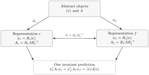
One abstract pair $|\psi\rangle,A$ can be represented in different orthonormal bases. The coordinate columns and matrices change by the same overlap map $S$, while the scalar prediction remains invariant. A passive rewrite follows the horizontal arrow; it does not prepare a new state.

Same State, Different Bases

Consider a spin-1/2 system. Define the $z$-basis and $x$-basis kets by

$$|+x\rangle =\frac{|+z\rangle+|-z\rangle}{\sqrt2}, \qquad |-x\rangle =\frac{|+z\rangle-|-z\rangle}{\sqrt2}.$$

The abstract state $|+x\rangle$ has component columns

$$[|+x\rangle]_z =\frac{1}{\sqrt2} \begin{pmatrix} 1\\ 1 \end{pmatrix}, \qquad [|+x\rangle]_x =\begin{pmatrix} 1\\ 0 \end{pmatrix}.$$

It is a two-term superposition in the $z$ basis and a single basis vector in the $x$ basis. Therefore, the statement “the state is in a superposition” is incomplete unless the reference decomposition is specified.

What is basis independent?

The physical ray, normalization, inner products with other states, and all correctly transformed measurement probabilities are basis independent. The number and values of components are generally not. Even a component being zero is not invariant under an arbitrary basis change.

For example, measuring spin along $z$ gives

$$p(+z)=p(-z)=\frac12,$$

whereas measuring along $x$ gives $p(+x)=1$ and $p(-x)=0$. The change in probability here is caused by changing the measurement, not merely by rewriting the state. A passive basis change that rewrites both the state and the same measurement leaves the probability unchanged.

Same Observable, Different Matrices

An observable is an abstract self-adjoint operator, subject in infinite dimensions to the appropriate domain conditions. Its matrix depends on the basis.

For spin along $z$,

$$S_z=\frac{\hbar}{2} \left( |+z\rangle\langle+z| -|-z\rangle\langle-z| \right).$$

Its matrix in the $z$ basis is diagonal:

$$[S_z]_z =\frac{\hbar}{2} \begin{pmatrix} 1&0\\ 0&-1 \end{pmatrix}.$$

In the ordered $x$ basis $\{|+x\rangle,|-x\rangle\}$, the same operator has matrix

$$[S_z]_x =\frac{\hbar}{2} \begin{pmatrix} 0&1\\ 1&0 \end{pmatrix}.$$

The first matrix does not describe a more real observable. It is convenient because the chosen basis diagonalizes $S_z$. The spectrum $\{+\hbar/2,-\hbar/2\}$ is unchanged.

Spectral information and coordinates

For a finite-dimensional operator, a unitary similarity transformation $A_f=SA_eS^\dagger$ preserves

$$\operatorname{Tr}A, \qquad \det A, \qquad \operatorname{spec}(A),$$

as well as rank and polynomial identities. Matrix entries, diagonal form, and individual eigenvector coordinates depend on the basis. Degenerate eigenspaces are invariant, but a particular orthonormal basis chosen inside a degenerate eigenspace is not unique.

Operator Representations compares matrix, multiplication, differential, and spectral forms in detail.

Hamiltonian in Energy and Position Representations

The harmonic oscillator gives a clean example of one operator with radically different-looking representations. Abstractly,

$$H=\frac{P^2}{2m}+\frac12m\omega^2X^2.$$

In its normalized energy eigenbasis $\{|n\rangle\}_{n=0}^\infty$,

$$\langle n|H|m\rangle =E_n\delta_{nm}, \qquad E_n=\hbar\omega\left(n+\frac12\right).$$

Thus the Hamiltonian is represented by an infinite diagonal matrix. In the position representation, the same operator acts on suitable wavefunctions as

$$(H\psi)(x) =\left[ -\frac{\hbar^2}{2m}\frac{d^2}{dx^2} +\frac12m\omega^2x^2 \right]\psi(x).$$

The diagonal matrix and the differential operator are not two Hamiltonians. They are related by the change from the energy basis to the generalized position representation. The eigenvalue equation

$$H|n\rangle=E_n|n\rangle$$

becomes the differential equation

$$\left[ -\frac{\hbar^2}{2m}\frac{d^2}{dx^2} +\frac12m\omega^2x^2 \right]\psi_n(x) =E_n\psi_n(x),$$

where $\psi_n(x)=\langle x|n\rangle$. The canonical solution belongs to Quantum Harmonic Oscillator; the point here is representation, not the spectrum’s derivation.

Position and Momentum Wavefunctions

For a particle on a line, the same abstract ket can be represented by

$$\psi(x)=\langle x|\psi\rangle, \qquad \phi(p)=\langle p|\psi\rangle.$$

With the site’s Fourier convention,

$$\phi(p) =\frac{1}{\sqrt{2\pi\hbar}} \int_{-\infty}^{\infty} e^{-ipx/\hbar}\psi(x)\,dx,$$

and

$$\psi(x) =\frac{1}{\sqrt{2\pi\hbar}} \int_{-\infty}^{\infty} e^{ipx/\hbar}\phi(p)\,dp.$$

The two functions carry the same state information when the transform exists in the appropriate sense. Their pointwise shapes and dimensions differ: $\psi(x)$ has units of length$^{-1/2}$, whereas $\phi(p)$ has units of momentum$^{-1/2}$. Their norms agree by unitarity of the Fourier transform,

$$\int |\psi(x)|^2\,dx =\int |\phi(p)|^2\,dp =1.$$

Position and momentum observables exchange simple and differential forms:

Abstract operator	Position representation	Momentum representation
$X$	multiplication by $x$	$i\hbar\,d/dp$
$P$	$-i\hbar\,d/dx$	multiplication by $p$

These formulas require suitable domains and boundary behavior. The continuous “bases” $|x\rangle$ and $|p\rangle$ are generalized eigenvectors rather than normalizable Hilbert-space vectors. Wavefunctions as Representations and Momentum-Space Representation own the detailed treatment.

Global Phase and Physical Equivalence

Normalized kets that differ only by a common phase represent the same pure state:

$$|\psi\rangle\sim e^{i\chi}|\psi\rangle.$$

The phase cancels from the rank-one density operator,

$$e^{i\chi}|\psi\rangle \langle\psi|e^{-i\chi} =|\psi\rangle\langle\psi|,$$

and therefore from every Born probability. The physical pure-state space is projective Hilbert space, the set of rays rather than normalized vectors.

Relative phase is different. For

$$|\psi_\varphi\rangle =\frac{|0\rangle+e^{i\varphi}|1\rangle}{\sqrt2},$$

changing $\varphi$ changes the ray unless the change is an integer multiple of $2\pi$. An interference-basis measurement can detect it. Multiplying the entire ket by $e^{i\chi}$ is a redundant representative choice; multiplying only one component changes the physical state relative to the chosen basis.

Rays and Global Phase is the canonical home for the equivalence relation and its projective geometry.

One Density Operator, Many Ensembles

Representation redundancy is not limited to bases. A mixed state can admit different ensemble decompositions. For a qubit,

$$\frac{I}{2} =\frac12|0\rangle\langle0| +\frac12|1\rangle\langle1|$$

and also

$$\frac{I}{2} =\frac12|+\rangle\langle+| +\frac12|-\rangle\langle-|.$$

No measurement on the qubit alone can distinguish these two unlabelled preparation ensembles because both assign the same density operator. The ensemble list is therefore not an intrinsic decomposition of $I/2$.

This statement has an important boundary. If the preparation choice is stored in an accessible classical register $C$, the joint classical–quantum state

$$\rho_{CQ} =\sum_j q_j|j\rangle\langle j|_C \otimes|\psi_j\rangle\langle\psi_j|_Q$$

retains information about the decomposition. Discarding $C$ produces the reduced state $\rho_Q$. Thus “same density operator” means operationally equivalent for measurements on the declared system, not identical laboratory histories with every record included.

See Ensembles and Preparation Procedures for the canonical distinction.

Passive Rewrites and Active Transformations

The same unitary matrix can describe either a passive change of coordinates or an active physical transformation. The distinction is semantic and operational.

Question	Passive description	Active description
What changes?	basis or coordinate labels	state, apparatus, or physical system
What stays fixed?	abstract physical situation	chosen basis or reference apparatus
Typical state formula	$\psi' = U^\dagger\psi$ in one convention	$
Can a fixed measurement probability change?	no, if all representations are transformed	yes, if the state changes relative to the fixed measurement

Spin example

Suppose a Stern–Gerlach apparatus measures $S_z$ and the input is $|+z\rangle$. An active rotation about $y$ by angle $\theta$ prepares

$$|\psi_\theta\rangle =e^{-i\theta S_y/\hbar}|+z\rangle.$$

Keeping the apparatus fixed, the probability of the $+z$ outcome becomes

$$p(+z\mid\theta) =|\langle+z|\psi_\theta\rangle|^2 =\cos^2\!\left(\frac{\theta}{2}\right).$$

This is a physical change. By contrast, rewriting the original state and the same $S_z$ measurement in the $x$ basis changes their arrays but leaves the certainty of the $+z$ outcome intact.

The full convention analysis belongs to Active and Passive Transformations.

Gauge Redundancy Is a Different Equivalence

A gauge description uses variables with deliberate redundancy. In electromagnetic quantum mechanics, potentials transform as

$$\mathbf A' =\mathbf A+\boldsymbol\nabla\chi, \qquad \Phi' =\Phi-\frac{\partial\chi}{\partial t}.$$

For a particle of charge $q$ using the corresponding sign convention, the wavefunction transforms as

$$\psi'(\mathbf r,t) =\exp\!\left[ \frac{iq}{\hbar}\chi(\mathbf r,t) \right] \psi(\mathbf r,t).$$

Potentials and wavefunction change together so that electric and magnetic fields, probability density, and gauge-covariant dynamics are unchanged. This is not merely a change from a $z$ basis to an $x$ basis, and it is not an active operation that moves a fixed state relative to a fixed apparatus. It is a redundancy in the variables used to represent the coupled matter–field description.

Global phase is gauge-like in the simpler projective sense that many normalized kets represent one ray. Electromagnetic gauge freedom is local and also transforms the potentials. The two ideas are related by phase structure but should not be identified without the gauge field and its transformation law.

Gauge Transformations in Quantum Mechanics owns the covariance calculation and the distinction between gauge redundancy and ordinary symmetry.

Pictures of Motion as Equivalent Bookkeeping

The Schrödinger and Heisenberg pictures distribute time dependence differently. For evolution $U(t,t_0)$,

$$\rho_S(t) =U(t,t_0)\rho_0U^\dagger(t,t_0), \qquad A_H(t) =U^\dagger(t,t_0)A_SU(t,t_0).$$

The Schrödinger picture evolves the state and keeps a time-independent observable fixed when it has no explicit time dependence. The Heisenberg picture keeps the reference state fixed and evolves the observable. Their prediction agrees:

$$\operatorname{Tr}[\rho_S(t)A_S] =\operatorname{Tr}[\rho_0A_H(t)].$$

This is not an ordinary spatial basis change, yet it illustrates the same discipline: identify what is representation-dependent and verify the invariant prediction. The interaction picture introduces a third useful distribution of time dependence. Pictures of Motion Overview gives the canonical map and links to full derivations.

Equivalent Formulations and Model Boundaries

Matrix mechanics, wave mechanics, and abstract Hilbert-space quantum mechanics can encode the same nonrelativistic predictions when their domains and transformations are handled correctly. Density operators extend rather than contradict pure-state notation. Path-integral and operator formulations can also agree within their common domains.

Equivalence must be demonstrated, not declared from visual resemblance. A translation dictionary should identify:

1. the state space and allowed states;
2. observables or measurement rules;
3. the dynamical law;
4. the map between descriptions;
5. the class of predictions shown to agree;
6. assumptions and domains on which the map is valid.

Two effective models can give nearly equal predictions in a restricted regime without being exact representations of one abstract theory. Conversely, two expressions can look different while being exactly related by a unitary change of representation. Equivalent Formulations develops this boundary.

Invariants to Check

When moving between equivalent orthonormal representations, useful checks include:

Quantity	Invariant statement
Norm	$\psi^\dagger\psi=\langle\psi
Transition probability	$
Born probability	$\operatorname{Tr}(\rho E_a)$ is unchanged
Expectation value	$\operatorname{Tr}(\rho A)$ is unchanged
Operator spectrum	unitary similarity preserves eigenvalues and multiplicities
Commutator structure	$[A',B']=U[A,B]U^\dagger$
Density-operator purity	$\operatorname{Tr}(\rho^2)$ is unchanged
Entropy	$-\operatorname{Tr}(\rho\log\rho)$ depends only on eigenvalues

Agreement of one invariant is necessary but may not establish full equivalence. For example, equal spectra do not by themselves identify which operator corresponds to which physical measurement, and equal expectation values for one state do not prove equality of two operators.

Infinite-Dimensional Caveats

In finite dimensions every orthonormal basis change is represented by a unitary matrix and all linear operators are bounded and everywhere defined. In wave mechanics:

• coordinate representations may use generalized eigenvectors and distributions;
• unbounded operators require domains that transform with the operator;
• boundary conditions can distinguish different self-adjoint operators sharing the same differential expression;
• traces and matrix elements may fail to exist unless their hypotheses are checked;
• an integral transform can be unitary on $L^2$ even when pointwise formulas require a limiting interpretation.

Thus a formal expression such as $A'=UAU^\dagger$ is incomplete unless $U$ also maps the relevant domain of $A$ onto the domain of $A'$. The accessible overview is Finite- vs Infinite-Dimensional Quantum Mechanics; rigorous operator theory lives in Mathematical Quantum Mechanics.

A Representation Audit

Before interpreting a formula, ask:

1. Abstract object: What state, operator, channel, or observable is being represented?
2. Representation map: Which basis, coordinates, gauge, or picture were chosen?
3. Convention: How is the transformation matrix defined, and where do its inverse or adjoint appear?
4. Physical operation: Is anything in the laboratory actively changed, or is this only a passive rewrite?
5. Invariant: Which probability, expectation value, spectrum, or correlation must remain unchanged?
6. Redundancy: Are multiple mathematical representatives intentionally identified, as with rays or gauge variables?
7. Domain: In infinite dimensions, are operator domains and boundary conditions included?
8. Model scope: Is the claimed equivalence exact, or only an approximation in a stated regime?

This audit often resolves apparent paradoxes before any calculation begins.

Common Mistakes

• Saying a state “is” a column vector without naming the basis.
• Changing state components but leaving the matrix of the same measurement in the old basis.
• Treating the diagonal representation of an operator as more physical than a nondiagonal one.
• Calling a state “a superposition” without specifying the reference basis or decomposition.
• Concluding that relative phase is unobservable because global phase is redundant.
• Confusing an active rotation of the state with a passive rotation of axes.
• Calling every unitary transformation a symmetry of the Hamiltonian.
• Treating gauge transformations as laboratory operations between distinct physical states.
• Treating one ensemble decomposition as an intrinsic list of states present in a mixed density operator.
• Assuming equal spectra imply that two operators have the same physical meaning.
• Forgetting that generalized position and momentum kets are not normalizable vectors.
• Transforming an unbounded operator formula without transforming its domain.

Connections

• The Minimal Language of Quantum Mechanics identifies the abstract objects whose representations are compared here.
• Bases and Representations introduces coordinate columns and operator matrices.
• Change of Basis derives the site’s passive convention and its invariants.
• Representation Translation Table provides a compact lookup across bra–ket, matrix, wavefunction, and density- operator notation.
• Active and Passive Transformations resolves rotation and translation sign conventions.
• Gauge Transformations in Quantum Mechanics develops local phase redundancy with electromagnetic potentials.
• Pictures of Motion Overview shows how equivalent dynamical bookkeeping preserves expectation values.

References

1. P. A. M. Dirac, The Principles of Quantum Mechanics, 4th ed., Oxford University Press, 1958. See Chapters I–III for transformations, representations, and bra–ket notation.
2. J. von Neumann, Mathematical Foundations of Quantum Mechanics, Princeton University Press, 1955. See Chapters II–III for Hilbert-space objects, spectral theory, and statistical operators.
3. R. Shankar, Principles of Quantum Mechanics, 2nd ed., Springer, 1994. See Chapters 1 and 4 for vector spaces, basis changes, and the quantum postulates.
4. J. J. Sakurai and J. Napolitano, Modern Quantum Mechanics, 3rd ed., Cambridge University Press, 2020. See Chapters 1–2 for representations, pictures of motion, and symmetry transformations.
5. A. Peres, Quantum Theory: Concepts and Methods, Kluwer, 1995. See Chapters 2–4 for preparations, states, tests, and composite descriptions.
6. L. E. Ballentine, Quantum Mechanics: A Modern Development, 2nd ed., World Scientific, 2014. See Chapters 2–4 for states, representations, and ensembles.
7. M. Reed and B. Simon, Methods of Modern Mathematical Physics, Vol. I: Functional Analysis, revised ed., Academic Press, 1980. See Chapters VII– VIII for unitary maps and self-adjoint operators.
8. C. Cohen-Tannoudji, B. Diu, and F. Laloë, Quantum Mechanics, Vol. 1, Wiley, 1977. See Complement A and Chapters II–III for representations and changes of basis.
9. B. C. Hall, Quantum Theory for Mathematicians, Springer, 2013. See Chapters 6–9 for Hilbert-space states, observables, and representations.

Exercises

1. Spin basis change. Write $|-z\rangle$ in the $x$ basis and verify its normalization. Then compute the probability of a $+z$ result using the $x$- basis matrices for both state and projector.

Solution

From the definitions,

$$|-z\rangle =\frac{|+x\rangle-|-x\rangle}{\sqrt2},$$

so in the ordered $x$ basis its column is

$$\psi_x =\frac1{\sqrt2} \begin{pmatrix} 1\\ -1 \end{pmatrix}.$$

Its norm is one. The $+z$ projector has $x$-basis matrix

$$[P_{+z}]_x =\frac12 \begin{pmatrix} 1&1\\ 1&1 \end{pmatrix}.$$

Therefore

$$\psi_x^\dagger[P_{+z}]_x\psi_x=0,$$

as required for the abstract orthogonality $\langle+z|-z\rangle=0$.

2. Operator invariants. Let

   $$A=\begin{pmatrix}2&1\\1&2\end{pmatrix}, \qquad S=\frac1{\sqrt2} \begin{pmatrix}1&1\\1&-1\end{pmatrix}.$$

   Compute $A'=SAS^\dagger$ and verify that trace, determinant, and spectrum are unchanged.

Solution

Direct multiplication gives

$$A' =\begin{pmatrix}3&0\\0&1\end{pmatrix}.$$

Both matrices have trace $4$, determinant $3$, and eigenvalues $3$ and $1$. The transformation reveals the eigenbasis but does not alter the abstract operator.

3. Energy and position forms. For a harmonic-oscillator energy eigenstate $|n\rangle$, show that $\langle H\rangle=E_n$ in both the energy and position representations. State the assumption needed for the position-space integration by parts.

Solution

In the energy basis,

$$\langle n|H|n\rangle=E_n.$$

In position space, $H\psi_n=E_n\psi_n$, so normalization gives

$$\int_{-\infty}^{\infty} \psi_n^*(x)(H\psi_n)(x)\,dx =E_n\int|\psi_n(x)|^2\,dx =E_n.$$

If one rewrites the kinetic term as an integral of $|\psi_n'|^2$, the wavefunction and derivative must decay sufficiently fast that the boundary term vanishes. More generally, $\psi_n$ must lie in the self-adjoint domain of $H$.

4. Fourier invariance. Use the momentum representation to show that the expectation value of momentum can be written either as

   $$\int\psi^*(x) \left(-i\hbar\frac{d}{dx}\right) \psi(x)\,dx$$

   or as $\int p|\phi(p)|^2\,dp$, assuming the required regularity and decay.

Solution

Insert the inverse Fourier transform for $\psi$. Acting with $-i\hbar d/dx$ on $e^{ipx/\hbar}$ produces $p$. The $x$ integral then gives $2\pi\hbar\,\delta(p-p')$, leaving

$$\langle P\rangle =\int_{-\infty}^{\infty} p|\phi(p)|^2\,dp.$$

The two integrals are the same abstract matrix element $\langle\psi|P|\psi\rangle$ in different representations.

5. Global versus relative phase. Compare $|\psi\rangle=(|0\rangle+|1\rangle)/\sqrt2$, $|\psi'\rangle=i|\psi\rangle$, and $|\chi\rangle=(|0\rangle+i|1\rangle)/\sqrt2$. Which pairs define the same ray? Find a measurement that distinguishes $|\psi\rangle$ from $|\chi\rangle$.

Solution

$|\psi'\rangle$ differs from $|\psi\rangle$ by a common phase and defines the same ray. No common phase maps $|\psi\rangle$ to $|\chi\rangle$, so they are different rays.

Measure in the $x$ basis. For $|\psi\rangle=|+\rangle$, the $+$ outcome has probability one. For $|\chi\rangle$,

$$|\langle+|\chi\rangle|^2 =\left|\frac{1+i}{2}\right|^2 =\frac12.$$

6. Two ensemble decompositions. Verify both decompositions of $I/2$ given on this page. Explain why retaining a classical preparation label can make the laboratory procedures distinguishable even though the reduced qubit state is the same.

Solution

Using $|\pm\rangle=(|0\rangle\pm|1\rangle)/\sqrt2$, the off-diagonal terms cancel:

$$\frac12|+\rangle\langle+| +\frac12|-\rangle\langle-| =\frac12 \begin{pmatrix}1&0\\0&1\end{pmatrix} =\frac I2.$$

The computational-basis mixture gives the same matrix directly. If an accessible register records which member was prepared, joint measurements can condition on that label. Tracing out or ignoring the register removes this information and leaves $I/2$ on the qubit.

7. Active or passive? A spin initially in $|+z\rangle$ is acted on by $U=e^{-i\pi S_y/(2\hbar)}$. First interpret $U$ actively with a fixed $S_z$ apparatus. Then interpret the corresponding unitary passively as a basis rewrite of both state and apparatus. What happens to the $+z$ probability in each case?

Solution

Actively, the state rotates to $|+x\rangle$ up to the convention’s overall phase. A fixed $S_z$ measurement then gives

$$p(+z)=\frac12.$$

Passively, the abstract state and apparatus are unchanged; only their arrays are rewritten in rotated coordinates. Transforming both consistently leaves the original prediction $p(+z)=1$. The same unitary algebra supports two different physical stories.

8. Picture independence. Let $\rho_0$ be any finite-dimensional density operator, $A$ an observable, and $U(t)$ unitary. Prove directly that the Schrödinger- and Heisenberg-picture expectation values agree. Why is this more than equality of operator spectra?

Solution

Using cyclicity of the trace,

$$\begin{aligned} \operatorname{Tr}[\rho_S(t)A] &=\operatorname{Tr}[U\rho_0U^\dagger A]\\ &=\operatorname{Tr}[\rho_0U^\dagger AU]\\ &=\operatorname{Tr}[\rho_0A_H(t)]. \end{aligned}$$

The equality matches the state, observable, and time dependence in the two descriptions for every $\rho_0$ and $A$. Equal spectra alone would not establish that full prediction dictionary.