Dirac’s Transformation Theory

Matrix mechanics and wave mechanics first looked like different theories. Matrix mechanics used arrays of transition quantities; wave mechanics used differential equations for wavefunctions. Dirac’s transformation theory helped reveal a deeper unity: both are representations of the same quantum structure.

In modern language, a state is not identical with any one column vector or wavefunction. A representation is a way of writing the state relative to a chosen basis or complete set of observables. Dirac’s transformation theory made that idea central.

Need for Unifying Formulations

By 1926, quantum mechanics had several successful languages:

• Heisenberg’s matrix mechanics emphasized transition quantities and noncommutative products.
• Born and Jordan’s formulation clarified the matrix algebra and canonical commutators.
• Schrödinger’s wave mechanics described systems by wavefunctions and differential equations.
• Born’s probability interpretation connected amplitudes to observed frequencies.

The urgent problem was not only to show that these languages gave the same spectra in examples. It was to understand why they were the same theory.

Dirac’s contribution was to treat transformations between descriptions as part of the theory itself. Instead of asking whether the matrix or wave picture was more real, transformation theory asks how to pass between representations without changing the underlying physical state.

Transformation Theory

In finite-dimensional modern notation, let $\{\lvert a\rangle\}$ and $\{\lvert b\rangle\}$ be two orthonormal bases. A state $\lvert\psi\rangle$ has components

$$\psi_a = \langle a\vert\psi\rangle, \qquad \psi_b = \langle b\vert\psi\rangle.$$

The overlap between bases is the transformation amplitude

$$S_{ba} = \langle b\vert a\rangle.$$

Then

$$\psi_b = \sum_a \langle b\vert a\rangle \psi_a.$$

The same idea works for continuous representations, with sums replaced by integrals. Position and momentum wavefunctions are related by a transformation kernel:

$$\psi(x) = \langle x\vert\psi\rangle, \qquad \phi(p) = \langle p\vert\psi\rangle.$$

With a common convention,

$$\langle x\vert p\rangle = \frac{1}{\sqrt{2\pi\hbar}} e^{ipx/\hbar},$$

so

$$\psi(x) = \int_{-\infty}^{\infty} \langle x\vert p\rangle \phi(p)\,dp.$$

The kernel is not a new physical wave by itself. It is a transformation amplitude between two representations.

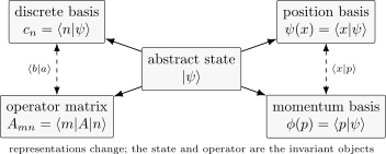
Dirac’s transformation viewpoint separates the abstract state from its representations. Matrix components, wavefunctions, and overlap kernels are different ways of expressing the same underlying quantum object.

States, Representations, and Observables

Transformation theory points toward the modern state-observable language. A state can be represented in the eigenbasis of an observable $A$, in the eigenbasis of another observable $B$, or in a continuous position or momentum representation. The physical state is the invariant object behind those coordinate descriptions.

For a discrete nondegenerate observable $A$, the modern spectral form is

$$A = \sum_a a\, \lvert a\rangle\langle a\rvert.$$

The amplitude for finding outcome $a$ in state $\lvert\psi\rangle$ is

$$\langle a\vert\psi\rangle,$$

and the probability is

$$P(a) = \lvert\langle a\vert\psi\rangle\rvert^2.$$

For another observable $B$, the relevant amplitudes are instead $\langle b\vert\psi\rangle$. The transformation amplitudes $\langle b\vert a\rangle$ tell how the two descriptions are related.

This is why representation changes are not optional bookkeeping. They are how quantum mechanics expresses incompatible measurement contexts, alternative bases, and equivalent formulations.

Bridge to Bra-Ket Notation

Dirac’s later bra-ket notation packages the transformation viewpoint compactly:

• a ket $\lvert\psi\rangle$ denotes the state vector;
• a bra $\langle a\rvert$ extracts an amplitude in the $a$ representation;
• an inner product $\langle a\vert\psi\rangle$ is a component or transition amplitude;
• an outer product $\lvert a\rangle\langle a\rvert$ is a projector in the nondegenerate discrete case.

Historically, the notation and the conceptual framework matured over time. It is still useful to read the notation as a compact summary of transformation theory: kets are not column vectors until a basis is chosen, and bras are not merely decorative row symbols. They encode the dual pairing that produces amplitudes.

For the working convention, see Bra-Ket Notation. For the mathematical translation, see Dirac Notation as Linear Algebra.

Bridge to Later Operator Formalism

Transformation theory also explains why later operator and field-theory languages could be representation-flexible. In operator quantum mechanics, the central objects are states, observables, amplitudes, and transformations. A coordinate-space wavefunction, an energy-basis column vector, and a momentum-space amplitude are different representations, not different physical theories.

This becomes especially important in more advanced settings:

• the Heisenberg picture moves time dependence into operators;
• scattering theory studies transition amplitudes between asymptotic states;
• path integrals compute kernels such as $\langle x_f,t_f\vert x_i,t_i\rangle$;
• quantum field theory organizes states and operators in Fock-space and field representations.

The historical bridge should not be overstated. Dirac’s transformation theory did not by itself provide all later mathematical rigor or all quantum-field-theoretic machinery. But it gave a durable conceptual grammar: choose a representation when useful, transform when necessary, and keep the representation-independent object in view.

What This Page Does Not Settle

Transformation theory clarified equivalence and notation, but it did not remove every subtlety. Continuous bases require generalized eigenvectors and distributions. Unbounded operators require domains. Measurements require probability rules and state-update models. Infinite systems and quantum fields can have inequivalent representations.

Those caveats are not failures of the transformation idea. They are reminders that the clean finite-dimensional formulas are ideal guides, not the whole mathematical story.

Common Mistakes

• Treating the wavefunction as the state itself rather than a representation of the state.
• Treating a matrix as the operator itself without specifying the basis.
• Thinking transformation theory is only about time evolution. It is also about changing representation.
• Forgetting that $\langle b\vert a\rangle$ is an amplitude, not a classical conditional probability.
• Applying finite-dimensional basis formulas to continuous spectra without distributional care.
• Reading modern bra-ket notation back into every 1920s paper as if it was already standardized.

Cross-Links

• Matrix Mechanics and Operator Ideas
• Heisenberg’s Matrix Mechanics
• Born and Jordan’s Matrix Formulation
• Observables Before Operators
• Commutation Relations in Historical Context
• Equivalence of Matrix and Wave Mechanics
• Schrödinger’s Wave Mechanics
• Interpreting the Wavefunction
• Bra-Ket Notation
• Bases and Representations
• Change of Basis
• Wavefunctions as Representations
• Operator Representations
• Equivalent Formulations
• Why Path Integrals?
• QFT Bridge Index

References

• P. A. M. Dirac, “The fundamental equations of quantum mechanics,” Proceedings of the Royal Society A 109, 642-653, 1925, DOI: 10.1098/rspa.1925.0150.
• P. A. M. Dirac, “The physical interpretation of the quantum dynamics,” Proceedings of the Royal Society A 113, 621-641, 1927, DOI: 10.1098/rspa.1927.0012.
• P. A. M. Dirac, The Principles of Quantum Mechanics, 4th ed., Oxford University Press, 1958.
• B. L. van der Waerden, ed., Sources of Quantum Mechanics, Dover, 1968.
• M. Jammer, The Conceptual Development of Quantum Mechanics, 2nd ed., American Institute of Physics, 1989.
• J. Mehra and H. Rechenberg, The Historical Development of Quantum Theory, Springer, 1982-2001.

Exercises

1. Let $\{\lvert a\rangle\}$ and $\{\lvert b\rangle\}$ be orthonormal bases with $S_{ba}=\langle b\vert a\rangle$. Show that $\psi_b=\sum_a S_{ba}\psi_a$.

Solution

Insert the identity in the $a$ basis:

$$I = \sum_a \lvert a\rangle\langle a\rvert.$$

Then

$$\psi_b = \langle b\vert\psi\rangle = \sum_a \langle b\vert a\rangle \langle a\vert\psi\rangle = \sum_a S_{ba}\psi_a.$$

2. Using $\langle x\vert p\rangle=(2\pi\hbar)^{-1/2}e^{ipx/\hbar}$, write $\psi(x)$ in terms of $\phi(p)$.

Solution

The position-space wavefunction is obtained by inserting the momentum representation:

$$\psi(x) = \int_{-\infty}^{\infty} \langle x\vert p\rangle \phi(p)\,dp = \frac{1}{\sqrt{2\pi\hbar}} \int_{-\infty}^{\infty} e^{ipx/\hbar} \phi(p)\,dp.$$

3. Why is $\langle b\vert a\rangle$ not a classical conditional probability?

Solution

It is generally complex and can interfere with other amplitudes. A probability is obtained only after the relevant amplitudes have been combined and squared according to the Born rule. The quantity $\langle b\vert a\rangle$ is therefore a transformation amplitude, not an ordinary conditional probability.

4. Explain why calling $\psi(x)$ “the state” can be misleading.

Solution

$\psi(x)=\langle x\vert\psi\rangle$ is the position representation of the abstract state $\lvert\psi\rangle$. The same state can also be represented by momentum-space amplitudes, energy-basis components, or another basis. Calling $\psi(x)$ the state hides the basis dependence and can make representation changes look like physical changes.