Quantum Harmonic Oscillator

The one-dimensional quantum harmonic oscillator describes a degree of freedom displaced from a stable equilibrium and subject to a restoring force proportional to that displacement. Its Hamiltonian is

$$\hat H =\frac{\hat p^2}{2m} +\frac12m\omega^2\hat x^2, \qquad m>0,\quad \omega>0.$$

This model is unusually important for two separate reasons. It is an exactly solvable bound-state problem whose differential and algebraic solutions expose much of the structure of quantum mechanics. It is also the leading approximation to any smooth potential near a nondegenerate stable minimum. Molecular vibrations, trapped particles, lattice normal modes, electromagnetic modes, and free quantum fields all inherit oscillator mathematics.

This page is the physical overview. The complete wave-mechanics derivation belongs to Differential-Equation Solution, while the first algebraic derivation belongs to Ladder-Operator Solution: First Encounter.

Problem and Assumptions

The configuration space is the full real line, and states are square-integrable wavefunctions in $L^2(\mathbb R)$. In position representation,

$$\hat x=x, \qquad \hat p=-i\hbar\frac{d}{dx},$$

so the stationary Schrödinger equation is

$$\left[ -\frac{\hbar^2}{2m}\frac{d^2}{dx^2} +\frac12m\omega^2x^2 \right]\psi(x) =E\psi(x).$$

Because $V(x)\to+\infty$ as $\lvert x\rvert\to\infty$, all energy eigenstates are bound and the spectrum is purely discrete. There are no hard walls: acceptable eigenfunctions and their derivatives are smooth, decay at both infinities, and remain nonzero in the classically forbidden tails.

The potential is even, $V(-x)=V(x)$, so the Hamiltonian commutes with parity. In one dimension, bound-state energies are nondegenerate; each oscillator eigenstate can therefore be assigned a definite parity.

Natural Scales

The parameters $m$, $\omega$, and $\hbar$ determine a natural length,

$$\ell=\sqrt{\frac{\hbar}{m\omega}},$$

a natural momentum,

$$p_\ell=\frac{\hbar}{\ell}=\sqrt{m\hbar\omega},$$

and a natural energy, $\hbar\omega$. The dimensionless phase-space variables

$$\xi=\frac{x}{\ell}, \qquad \pi=\frac{\ell p}{\hbar}$$

satisfy $[\hat\xi,\hat\pi]=i$. The Hamiltonian then takes the parameter-free form

$$\frac{\hat H}{\hbar\omega} =\frac12\left(\hat\pi^2+\hat\xi^2\right),$$

or, in position representation,

$$\frac{\hat H}{\hbar\omega} =\frac12\left( -\frac{d^2}{d\xi^2}+\xi^2 \right).$$

All one-dimensional oscillators are therefore the same dimensionless eigenvalue problem. Changing $m$ or $\omega$ only rescales position, momentum, energy, and time. In particular, larger $m\omega$ squeezes the wavefunctions in position while broadening them in momentum.

The oscillator length is not the ground-state standard deviation. With the convention used here,

$$\Delta x_0=\frac{\ell}{\sqrt2}.$$

Some sources define their characteristic length as this standard deviation instead, so formulas should always be checked against the author’s convention.

Spectrum and Turning Points

The allowed energies are

$$E_n=\hbar\omega\left(n+\frac12\right), \qquad n=0,1,2,\ldots$$

and neighboring levels have the constant spacing

$$E_{n+1}-E_n=\hbar\omega.$$

The classical turning points at energy $E_n$ satisfy $V(x_{\mathrm t})=E_n$. Hence

$$x_{\mathrm t}^{(n)} =\pm\ell\sqrt{2n+1}.$$

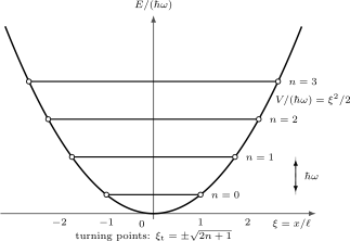
The oscillator levels are separated by $\hbar\omega$. Open circles mark the classical turning points $\xi_{\mathrm t}=\pm\sqrt{2n+1}$. The horizontal segments indicate the classically allowed intervals, not the support of the quantum states: every eigenfunction has exponentially decaying tails beyond those points.

The equal spacing is exact only for a perfectly quadratic potential. Anharmonic corrections generally make transition frequencies depend on $n$. The absence of degeneracy is also specific to the one-dimensional problem; multidimensional isotropic oscillators can have several independent states at the same total energy.

Energy Eigenfunctions

The normalized position-space eigenfunctions are

$$\psi_n(x) =\frac{1}{\sqrt{2^n n!}} \left(\frac{1}{\pi\ell^2}\right)^{1/4} H_n\left(\frac{x}{\ell}\right) \exp\left(-\frac{x^2}{2\ell^2}\right),$$

where $H_n$ is the physicists’ Hermite polynomial. Equivalently,

$$\psi_n(x)=\ell^{-1/2}\phi_n(x/\ell),$$

where the dimensionless Hermite functions $\phi_n$ form an orthonormal basis of $L^2(\mathbb R)$. Their identities, Fourier-transform behavior, and recurrence relations are collected in Hermite Functions.

The first three states are

$$\begin{aligned} \psi_0(x) &=\frac{1}{\pi^{1/4}\sqrt{\ell}}\, e^{-x^2/(2\ell^2)},\\ \psi_1(x) &=\frac{\sqrt2\,x}{\pi^{1/4}\ell^{3/2}}\, e^{-x^2/(2\ell^2)},\\ \psi_2(x) &=\frac{2x^2/\ell^2-1} {\sqrt2\,\pi^{1/4}\sqrt{\ell}}\, e^{-x^2/(2\ell^2)}. \end{aligned}$$

Their qualitative structure follows general one-dimensional bound-state theory:

• $\psi_n$ is real up to an overall phase.

• It has parity $(-1)^n$:

  $$\psi_n(-x)=(-1)^n\psi_n(x).$$

• It has exactly $n$ simple nodes on the real line.

• Its largest-scale oscillations lie between the classical turning points, but its tails extend outside them.

• Increasing $n$ increases both the spatial extent and the number of oscillations.

The position probability density of an energy eigenstate is stationary:

$$\lvert\Psi_n(x,t)\rvert^2 =\left\lvert e^{-iE_nt/\hbar}\psi_n(x) \right\rvert^2 =\lvert\psi_n(x)\rvert^2.$$

Stationarity does not mean that kinetic energy vanishes or that the particle sits still. It means that all time dependence is a global phase for that state.

Zero-Point Energy

The lowest energy is

$$E_0=\frac12\hbar\omega,$$

not zero. A rough uncertainty argument already gives the correct scale. Localizing a state to width $\Delta x$ requires $\Delta p\gtrsim\hbar/(2\Delta x)$, so

$$\langle H\rangle \gtrsim \frac{\hbar^2}{8m(\Delta x)^2} +\frac12m\omega^2(\Delta x)^2.$$

The competing terms prevent both kinetic and potential energy from vanishing. Minimizing this estimate gives $\Delta x=\ell/\sqrt2$ and $\langle H\rangle\ge\hbar\omega/2$; the Gaussian ground state attains the bound. Zero-Point Energy develops the exact operator argument and the limits of its physical interpretation.

Adding a constant $C$ to this single-particle Hamiltonian shifts every energy to $E_n+C$ without changing any state or transition frequency. What is invariant within the isolated model is the spacing. Absolute zero-point energies matter when gravity, changing boundary conditions, or comparisons between inequivalent Hamiltonians make the energy offset physically consequential.

Moments, Uncertainty, and the Virial Theorem

Parity immediately gives

$$\langle x\rangle_n=0, \qquad \langle p\rangle_n=0.$$

The second moments are

$$\langle x^2\rangle_n =\left(n+\frac12\right)\ell^2,$$

and

$$\langle p^2\rangle_n =\left(n+\frac12\right)m\hbar\omega.$$

Consequently,

$$\Delta x_n\,\Delta p_n =\hbar\left(n+\frac12\right).$$

Only the ground state saturates the Heisenberg lower bound. For every stationary eigenstate, the quantum virial theorem gives equal mean kinetic and potential energies:

$$\left\langle\frac{\hat p^2}{2m}\right\rangle_n = \left\langle\frac12m\omega^2\hat x^2\right\rangle_n =\frac{E_n}{2}.$$

These relations are strong diagnostics for analytic and numerical wavefunctions. A purported normalized eigenstate that violates them is not an oscillator eigenstate under the conventions above.

Matrix Elements and Selection Rule

Position and momentum connect only neighboring energy levels:

$$\langle m\vert\hat x\vert n\rangle =\frac{\ell}{\sqrt2} \left( \sqrt{n+1}\,\delta_{m,n+1} +\sqrt n\,\delta_{m,n-1} \right),$$ $$\langle m\vert\hat p\vert n\rangle =\frac{i\hbar}{\ell\sqrt2} \left( \sqrt{n+1}\,\delta_{m,n+1} -\sqrt n\,\delta_{m,n-1} \right).$$

Thus a perturbation proportional to $x$ has the oscillator selection rule $\Delta n=\pm1$. This is a statement about matrix elements, not an absolute ban on other transitions: nonlinear couplings such as $x^2$ have different selection rules, and anharmonic eigenstates need not obey the ideal-oscillator rule exactly.

The ladder-operator derivation makes these formulas almost immediate. Here they also provide a compact bridge between stationary states and observable oscillatory motion.

Time Evolution

An arbitrary initial state can be expanded in the energy basis:

$$\lvert\psi(0)\rangle =\sum_{n=0}^{\infty}c_n\lvert n\rangle, \qquad \sum_{n=0}^{\infty}\lvert c_n\rvert^2=1.$$

Its evolution is

$$\lvert\psi(t)\rangle =\sum_{n=0}^{\infty} c_n e^{-i\omega(n+1/2)t}\lvert n\rangle.$$

Because all relative frequencies are integer multiples of $\omega$, every normalizable oscillator state is cyclic with period

$$T=\frac{2\pi}{\omega}.$$

At $T$, the state acquires the common phase $-1$, so all rays and observables return exactly. At half a period,

$$e^{-i\hat H\pi/(\hbar\omega)} =-i\,\hat\Pi,$$

where $\hat\Pi$ is parity. The wavefunction therefore returns reflected about the origin, up to a global phase.

The Heisenberg equations are identical in form to the classical oscillator equations:

$$\frac{d\hat x}{dt}=\frac{\hat p}{m}, \qquad \frac{d\hat p}{dt}=-m\omega^2\hat x.$$

Their exact solution is

$$\begin{aligned} \hat x(t) &=\hat x(0)\cos\omega t +\frac{\hat p(0)}{m\omega}\sin\omega t,\\ \hat p(t) &=\hat p(0)\cos\omega t -m\omega\hat x(0)\sin\omega t. \end{aligned}$$

Taking expectation values shows that $\langle x\rangle$ and $\langle p\rangle$ follow the classical equations for every state, not only in a semiclassical limit. The state itself need not behave classically: energy eigenstates have zero mean displacement, squeezed states can change shape, and generic superpositions display interference.

Classical Correspondence

A classical oscillator of energy $E$ has continuous energy and oscillates between

$$x_{\mathrm t}=\sqrt{\frac{2E}{m\omega^2}}.$$

Sampling the orbit uniformly in time gives the classical position density

$$P_{\mathrm{cl}}(x) =\frac{1}{\pi\sqrt{x_{\mathrm t}^2-x^2}}, \qquad \lvert x\rvert<x_{\mathrm t}.$$

This density is largest near the turning points, where the classical speed is smallest. A high-$n$ quantum density has many rapid oscillations and penetrates slightly into the forbidden region. After averaging over spatial scales larger than the local fringe spacing, it approaches the classical distribution away from the turning-point boundary layers.

This is the relevant correspondence statement. Pointwise convergence of $\lvert\psi_n(x)\rvert^2$ does not occur because the oscillations become increasingly rapid rather than disappearing. Localized Coherent States provide a different classical limit: their probability packet follows the classical orbit without changing its width.

Why the Oscillator Is Universal

Let a smooth potential have a stable, nondegenerate minimum at $x_0$. Its Taylor expansion is

$$V(x) =V(x_0) +\frac12V''(x_0)(x-x_0)^2 +\frac{1}{3!}V^{(3)}(x_0)(x-x_0)^3 +\cdots,$$

because $V'(x_0)=0$. Identifying

$$\omega=\sqrt{\frac{V''(x_0)}{m}}$$

gives a harmonic oscillator at leading nonconstant order. The approximation is reliable when the states of interest occupy displacements small enough that the cubic and higher terms are perturbative over the relevant wavefunction support.

For several coupled coordinates, a quadratic expansion produces a matrix of second derivatives. Diagonalizing the mass-weighted matrix separates the motion into independent normal modes, each of which is an oscillator. The method underlies Normal Modes of Polyatomics and the quantization of collective excitations.

The approximation can fail near a flat minimum, a barrier top, a strongly anharmonic region, or energies close to dissociation. A double well also cannot be globally replaced by one oscillator: local oscillators around the two minima miss tunneling between them.

Two Exact Solution Routes

The two standard derivations answer different questions:

1. Differential-Equation Solution scales the Schrödinger equation, extracts the Gaussian asymptotics, derives Hermite’s equation, and shows how square integrability selects the discrete energies.
2. Ladder-Operator Solution: First Encounter factorizes the Hamiltonian, proves that the number operator is nonnegative, and constructs the spectrum by raising a lowest state.

The first route makes boundary behavior and special functions explicit. The second exposes the spectrum-generating algebra and computes matrix elements efficiently. Neither is merely a shortcut for the other; together they explain why the oscillator is both a wave equation and an algebraic template.

Worked Scaling Example

Suppose the mass is increased by a factor of four while the angular frequency is held fixed. Then

$$\ell'=\sqrt{\frac{\hbar}{(4m)\omega}}=\frac{\ell}{2},$$

so every position-space eigenfunction is compressed horizontally by a factor of two. The energy levels are unchanged because they depend on $\omega$, not separately on $m$:

$$E_n'=\hbar\omega\left(n+\frac12\right)=E_n.$$

The momentum scale doubles,

$$p_\ell'=\sqrt{4m\hbar\omega}=2p_\ell.$$

This example separates three ideas often conflated in dimensional reasoning: the mass controls the spatial and momentum scales, the frequency controls both those scales and the level spacing, and normalization supplies the corresponding amplitude factor in position space.

Numerical Benchmark

The oscillator is an excellent test problem for discretization and eigensolver code because exact results are available. On a finite interval $[-L,L]$ with a spatial grid, a trustworthy computation should demonstrate convergence under both increasing $L$ and decreasing grid spacing.

Useful checks include:

• eigenvalues approach $\hbar\omega(n+1/2)$;
• numerical eigenvectors alternate in parity;
• the $n$th state has $n$ interior nodes;
• the virial ratio approaches one;
• the wavefunction is negligible before reaching the artificial boundaries;
• eigenvectors are orthonormal under the quadrature rule used by the discretization.

Agreement of a few eigenvalues alone is not sufficient. A box that is too small can accidentally give plausible low-lying energies while distorting tails and moments.

Common Mistakes

• Writing $E_n=n\hbar\omega$ and dropping the zero-point term.
• Starting the oscillator quantum number at $n=1$ rather than $n=0$.
• Confusing $\ell=\sqrt{\hbar/(m\omega)}$ with $\Delta x_0=\ell/\sqrt2$.
• Interpreting the classical turning points as quantum boundary conditions.
• Assuming an energy eigenstate represents a localized particle moving back and forth.
• Treating equal level spacing as a generic feature of all confining potentials.
• Calling $\hat a^\dagger$ a particle-creation operator in this single-particle problem; it raises oscillator excitation.
• Expecting the high-$n$ probability density to converge pointwise to the classical density.
• Applying the local quadratic approximation without checking the size of anharmonic terms over the occupied region.

Where This Is Used

• Hermite Polynomials supplies the special-function identities behind the differential solution.
• Number States develops the energy basis and occupation-number language.
• Displaced Oscillator shows that a linear force shifts the equilibrium without changing the level spacing.
• Squeezed States: First Encounter studies Gaussian states whose quadrature uncertainties are redistributed.
• Oscillator as a Universal Local Model develops the normal-mode and approximation viewpoint.
• Variational Estimate for the Harmonic Oscillator uses the exact ground state as a benchmark for variational reasoning.
• Vibrations of Diatomics applies the model to molecular spectra and identifies anharmonic corrections.
• Degeneracy in Separable Systems explains shell degeneracy for several identical oscillator coordinates.
• General Uncertainty Relations provides the uncertainty framework behind zero-point motion.
• Later quantum-matter, quantum-optics, and field-theory pages quantize independent normal modes as oscillators.

References

• D. J. Griffiths and D. F. Schroeter, Introduction to Quantum Mechanics, 3rd ed., Cambridge University Press, 2018, ch. 2.
• R. Shankar, Principles of Quantum Mechanics, 2nd ed., Springer, 1994, ch. 7.
• J. J. Sakurai and J. Napolitano, Modern Quantum Mechanics, 3rd ed., Cambridge University Press, 2020, sec. 2.3.
• C. Cohen-Tannoudji, B. Diu, and F. Laloë, Quantum Mechanics, vol. 1, Wiley, 1977, complement V A.
• L. D. Landau and E. M. Lifshitz, Quantum Mechanics: Non-Relativistic Theory, 3rd ed., Butterworth-Heinemann, 1977, sec. 23.

Exercises

1. Starting from the dimensional Schrödinger equation, use $\xi=x/\ell$ to derive the parameter-free Hamiltonian $\hat H/(\hbar\omega)$.

Solution

Because $\ell^2=\hbar/(m\omega)$,

$$\frac{d}{dx}=\frac{1}{\ell}\frac{d}{d\xi}.$$

The kinetic and potential terms become

$$-\frac{\hbar^2}{2m\ell^2}\frac{d^2}{d\xi^2} =-\frac{\hbar\omega}{2}\frac{d^2}{d\xi^2},$$

and

$$\frac12m\omega^2\ell^2\xi^2 =\frac{\hbar\omega}{2}\xi^2.$$

Therefore

$$\frac{\hat H}{\hbar\omega} =\frac12\left( -\frac{d^2}{d\xi^2}+\xi^2 \right).$$

2. Derive the turning points of the $n$th eigenstate. By what factor does their magnitude change from $n=0$ to $n=8$?

Solution

Set the potential equal to the eigenenergy:

$$\frac12m\omega^2x_{\mathrm t}^2 =\hbar\omega\left(n+\frac12\right).$$

Using $\ell^2=\hbar/(m\omega)$ gives

$$\lvert x_{\mathrm t}^{(n)}\rvert =\ell\sqrt{2n+1}.$$

The ratio is

$$\frac{\lvert x_{\mathrm t}^{(8)}\rvert} {\lvert x_{\mathrm t}^{(0)}\rvert} =\sqrt{17}.$$

3. Use the given second moments to verify the virial theorem and find the uncertainty product in $\lvert n\rangle$.

Solution

The kinetic expectation value is

$$\langle T\rangle_n =\frac{\langle p^2\rangle_n}{2m} =\frac{\hbar\omega}{2} \left(n+\frac12\right) =\frac{E_n}{2}.$$

Similarly,

$$\langle V\rangle_n =\frac12m\omega^2\langle x^2\rangle_n =\frac{\hbar\omega}{2} \left(n+\frac12\right) =\frac{E_n}{2}.$$

Since both first moments vanish,

$$\Delta x_n\Delta p_n =\sqrt{ \left(n+\frac12\right)\ell^2 \left(n+\frac12\right)m\hbar\omega } =\hbar\left(n+\frac12\right).$$

4. Let

$$\lvert\psi(0)\rangle =\frac{1}{\sqrt2} \left(\lvert0\rangle+e^{i\phi}\lvert1\rangle\right).$$

Find $\langle x\rangle(t)$ using $\langle0\vert\hat x\vert1\rangle=\ell/\sqrt2$.

Solution

The relative phase evolves at frequency $(E_1-E_0)/\hbar=\omega$. The diagonal position matrix elements vanish, so

$$\begin{aligned} \langle x\rangle(t) &=2\operatorname{Re}\left[ \frac{e^{i(\phi-\omega t)}}{2} \langle0\vert\hat x\vert1\rangle \right]\\ &=\frac{\ell}{\sqrt2}\cos(\phi-\omega t). \end{aligned}$$

The mean position follows a classical sinusoid even though the state is a coherent superposition of only two energies.

5. Prove that evolution through half a classical period is parity up to a global phase.

Solution

For $T/2=\pi/\omega$,

$$e^{-iE_nT/(2\hbar)} =e^{-i\pi(n+1/2)} =-i(-1)^n.$$

Because $\hat\Pi\lvert n\rangle=(-1)^n\lvert n\rangle$, both operators have the same action on every basis state:

$$e^{-i\hat HT/(2\hbar)}=-i\hat\Pi.$$

Thus $\psi(x,T/2)=-i\psi(-x,0)$.

6. A numerical calculation gives low-lying energies accurate to four digits, but $\langle T\rangle/\langle V\rangle=1.18$ for the computed ground state. What should be checked before accepting the result?

Solution

The exact ground state obeys $\langle T\rangle=\langle V\rangle$, so the moment calculation or the eigenvector is not converged even if the energy appears accurate. One should enlarge the interval, refine the grid or basis, verify the kinetic operator and quadrature weights, renormalize with the same discrete inner product, and confirm that the wavefunction is negligible at the artificial boundaries. Energies can converge faster than tails and derivative-sensitive observables.