Covariant Dirac Equation
The free Dirac equation for a four-component spinor is
It is first order in spacetime derivatives, yet its Clifford algebra ensures that every component satisfies the Klein–Gordon mass-shell equation. Lorentz covariance does not mean that is a four-vector: coordinates transform with , while spinor components transform with a matrix that intertwines with the gamma matrices. The resulting current has
which repairs the local-density problem of a one-particle Klein–Gordon amplitude. It does not remove the need for quantum fields when interactions can create particles and antiparticles.
Required background. Metric and Units, Four-Vectors, the Energy–Momentum Relation, Gamma Matrices, the Gamma-Matrix Conventions, and the Klein–Gordon Equation supply every convention and factorization used below.
Covariant operator and plane waves
Section titled “Covariant operator and plane waves”Define the free Dirac operator
For a constant spinor and the default plane wave,
the differential equation becomes the algebraic equation
Multiplying from the left by gives
A nonzero plane-wave spinor is therefore on shell. The matrix equation also constrains its four components; they are not four independent scalar wave amplitudes.
The negative-frequency solutions are part of the free equation. In a fixed- particle treatment they signal the second energy sector. In the quantized Dirac field, the corresponding mode operators acquire the antiparticle interpretation without retaining an unbounded-below many-particle energy.
Squaring gives Klein–Gordon componentwise
Section titled “Squaring gives Klein–Gordon componentwise”Multiply the equation by the conjugate algebraic factor:
The scalar mass commutes with the derivative operator, so the mixed terms cancel. Because partial derivatives commute,
The product is therefore
and each spinor component obeys
The converse is false. Four arbitrary Klein–Gordon solutions need not satisfy the first-order Dirac constraints. Squaring can introduce solutions of the second-order equation that the original factor does not annihilate.
Lorentz covariance as an intertwining relation
Section titled “Lorentz covariance as an intertwining relation”Let a proper orthochronous Lorentz transformation act on coordinates as
The spinor transforms as
where is chosen so that
The derivative transforms with the inverse Lorentz matrix:
Since is constant for a global inertial-frame change,
Hence
so a solution in one inertial frame maps to a solution in every other.
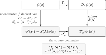
Lorentz covariance uses two linked representations. The vector matrix changes coordinates and derivatives; changes spinor components. The gamma-matrix intertwiner makes applying the Dirac operator before or after the transformation equivalent.
For transformations continuously connected to the identity, may be built from the generators . The exact exponential sign depends on the active/passive and parameter conventions, so the displayed intertwining identity is the authority used here.
The spinor representation is double valued over the Lorentz transformation: and induce the same . A spatial rotation changes a spinor’s sign, while bilinears and physical rays return to themselves. This is the local algebraic trace of the double cover of the proper orthochronous Lorentz group.
Adjoint equation and conserved current
Section titled “Adjoint equation and conserved current”The Dirac adjoint is
Take the Hermitian conjugate of the Dirac equation and use . The adjoint equation is
Multiplying the original equation on the left by gives
Multiplying the adjoint equation on the right by and adding cancels the mass terms:
Define
Then
The density is pointwise nonnegative and the spatial current is
For solutions that decay sufficiently fast, or obey boundary conditions with zero net flux, integrating the continuity equation gives conservation of .
The matrix eigenvalues of each are , and more generally . Thus the current is causal: its local flow speed does not exceed .
Hamiltonian form and initial data
Section titled “Hamiltonian form and initial data”Separate the time derivative and multiply by :
with
This is the canonical owner of the free Dirac Hamiltonian used by the compact Dirac Hamiltonian card. The formula alone is not a self-adjoint operator: a Hilbert space, spatial domain, and boundary conditions must also be specified. On , the standard free realization is self-adjoint on . The detailed domain, spectral projectors, unitary evolution, and boundary-form analysis are developed in The Dirac Hamiltonian as an Operator.
Because the equation is first order in time, initial data consist of
alone. Its time derivative is fixed by . Specifying an independent would generally overdetermine the problem.
In momentum space, , so its free spectrum contains the two branches . The positive density does not mean the negative-energy branch can be discarded locally without consequence; projection onto one branch is nonlocal in position space.
Fixed-particle scope and the QFT boundary
Section titled “Fixed-particle scope and the QFT boundary”The free Dirac equation and weak prescribed external fields support highly accurate first-quantized calculations when pair creation is negligible. They describe spin, relativistic kinematics, currents, atomic fine structure, and the controlled Pauli limit.
They are not a complete interacting relativistic quantum theory. When appreciable pair-production channels are open, fixed particle number fails. An energy scale comparable to the particle–antiparticle gap is a warning, not by itself a sufficient criterion: field geometry, invariants, duration, and transition rates also matter. Quantum electrodynamics promotes to an operator-valued field; both frequency sectors are then necessary for locality, causal propagation, and antiparticle excitations.
Independently, the finite-dimensional Lorentz boost matrix need not be unitary in the ordinary Euclidean component norm, even in free one-particle theory. The conserved Hilbert-space norm is an integral on a chosen spacelike slice, while covariant bilinears use the Dirac adjoint.
Continue with Free Dirac Spinors for normalized modes and completeness, The Dirac Current for the Gordon decomposition and spin current, and Dirac Equation as Bridge for the additional structure required by quantum field theory.
Common pitfalls
Section titled “Common pitfalls”Transforming a spinor as a four-vector. Four components do not determine the representation. Use and the gamma-matrix intertwiner.
Assuming for boosts. Spatial rotations are unitary in the finite spinor space; boosts are not. Covariant bilinears are preserved through , not a Euclidean component norm at one event.
Forgetting the transformed argument. Covariance requires , not merely multiplication of components at an unchanged coordinate label.
Inferring the Dirac equation from Klein–Gordon alone. Squaring loses the first-order constraint. Every Dirac solution is Klein–Gordon componentwise, but not every four-tuple of Klein–Gordon solutions is a Dirac solution.
Exercises
Section titled “Exercises”1. Operator factorization
Section titled “1. Operator factorization”Multiply the two Dirac factors and recover the Klein–Gordon equation with the shared metric convention.
Solution
The mass cross terms cancel, and commuting derivatives remove the gamma-commutator contribution:
Dividing the resulting equation by gives
2. Current conservation
Section titled “2. Current conservation”Derive the adjoint equation and use it to prove .
Solution
Hermitian conjugation followed by right multiplication with gives
Multiplying by and adding the original equation multiplied by cancels the mass terms and produces
3. Covariance check
Section titled “3. Covariance check”Starting from the derivative transformation and intertwining identity, prove .
Solution
Use
and contract with :
The mass term commutes with , so the full operator transforms in the stated way.
4. Hamiltonian form
Section titled “4. Hamiltonian form”Derive from the covariant equation.
Solution
Using , write
Multiply by and use , , and to obtain
References
Section titled “References”- P. A. M. Dirac, “The Quantum Theory of the Electron,” Proceedings of the Royal Society A 117, 610–624, 1928, doi:10.1098/rspa.1928.0023.
- W. Greiner, Relativistic Quantum Mechanics: Wave Equations, 3rd ed., Springer, 2000, doi:10.1007/978-3-662-04275-5.
- F. Schwabl, Advanced Quantum Mechanics, 3rd ed., Springer, 2005, doi:10.1007/3-540-28528-8.
- M. D. Schwartz, Quantum Field Theory and the Standard Model, Cambridge University Press, 2014, doi:10.1017/9781139540940.