Klein–Gordon Equation

The free Klein–Gordon equation is the direct wave-equation form of the relativistic mass shell for a scalar amplitude:

$$\boxed{ \left( \Box+\frac{m^2c^2}{\hbar^2} \right)\phi(x)=0 }.$$

It is Lorentz covariant, admits both frequency branches of $E^2=\mathbf p^2c^2+m^2c^4$, and is second order in time. These successes also expose a one-particle limitation: its natural conserved density is not positive definite. In quantum field theory the same equation becomes the equation of motion for a scalar field, and the conserved complex-field current is interpreted as charge rather than Born probability.

Required background. Metric and Units, Four-Vectors, and the Energy–Momentum Relation fix the differential signs, scalar contractions, mass shell, and frequency branches used below.

From the mass shell to a scalar wave equation

Start with

$$E^2-\mathbf p^2c^2-m^2c^4=0.$$

For the phase $e^{-i(Et-\mathbf p\cdot\mathbf x)/\hbar}$, use

$$E\longrightarrow i\hbar\partial_t, \qquad \mathbf p\longrightarrow-i\hbar\nabla.$$

Applying the operator polynomial to a complex scalar amplitude gives

$$\left[ -\hbar^2\partial_t^2 +\hbar^2c^2\nabla^2 -m^2c^4 \right]\phi=0.$$

Dividing by $-\hbar^2c^2$ yields

$$\left( \frac{1}{c^2}\partial_t^2 -\nabla^2 +\frac{m^2c^2}{\hbar^2} \right)\phi=0.$$

Because

$$\Box=\partial_\mu\partial^\mu = \frac{1}{c^2}\partial_t^2-\nabla^2,$$

the compact covariant form follows. In natural units it is simply

$$(\Box+m^2)\phi=0.$$

The amplitude is a Lorentz scalar: $\phi'(x')=\phi(x)$ for $x'=\Lambda x$. Since $\Box$ is a scalar operator and $m$ is invariant, the equation has the same form in every inertial frame.

Plane waves recover both mass-shell branches

Insert

$$\phi_p(x)=A e^{-ip\cdot x/\hbar} = A e^{-i(Et-\mathbf p\cdot\mathbf x)/\hbar}.$$

Then

$$\Box\phi_p = -\frac{p_\mu p^\mu}{\hbar^2}\phi_p,$$

so the equation becomes

$$(p^2-m^2c^2)\phi_p=0.$$

A nonzero mode therefore obeys

$$E=\pm\sqrt{\mathbf p^2c^2+m^2c^4}.$$

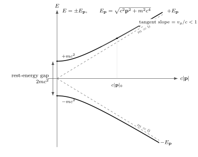
The Klein–Gordon equation retains both sheets of the mass shell because it is quadratic in the time derivative. The branch label is initially a frequency label; antiparticle interpretation requires the field-theory framework.

A general complex solution is a superposition of both frequency sectors. Reality imposes a relation between their coefficients rather than deleting one sector. For a real field, the coefficient of a negative-frequency mode is the complex conjugate of the corresponding positive-frequency coefficient. The precise momentum labels, coefficient reconstruction, and reality condition are worked out in Plane-Wave Solutions.

Second-order initial data

On an initial constant-time slice $t=t_0$, a Klein–Gordon solution is fixed by two functions,

$$\phi(t_0,\mathbf x), \qquad \partial_t\phi(t_0,\mathbf x),$$

subject to the regularity required by the chosen solution space. The equation then determines $\partial_t^2\phi$ and propagates both data forward and backward in time.

This differs from the Schrödinger and Dirac equations, which are first order in time and require only the state amplitude at $t_0$. Replacing the second- order equation by a positive square root removes one frequency branch but introduces a spatially nonlocal pseudodifferential operator. The local scalar equation and a one-branch Schrödinger evolution are not interchangeable descriptions.

For sufficiently regular compactly supported initial data, disturbances propagate within the Minkowski causal cone. That hyperbolic propagation fact does not by itself supply a positive probability density. For explicit evolution with a source, use Solving Scalar Initial-Value Problems.

Conserved current for a complex scalar

Let $\phi$ solve the Klein–Gordon equation and $\phi^*$ its complex conjugate. Multiply the equation for $\phi$ by $\phi^*$, multiply the conjugate equation by $\phi$, and subtract. The mass terms cancel:

$$\phi^*\Box\phi-\phi\Box\phi^*=0.$$

Using the product rule,

$$\partial_\mu \left( \phi^*\partial^\mu\phi -\phi\partial^\mu\phi^* \right)=0.$$

For $m>0$, one conventional normalization is

$$j^\mu = \frac{i\hbar}{2m} \left( \phi^*\partial^\mu\phi -\phi\partial^\mu\phi^* \right), \qquad \partial_\mu j^\mu=0.$$

The overall nonzero constant is conventional; conservation does not fix it. For $m=0$, use a fixed nonzero normalization scale instead of dividing by $m$. That change does not repair the sign indefiniteness. For the plane wave above,

$$j^\mu=\frac{p^\mu}{m}|A|^2, \qquad j^0=\frac{E}{mc}|A|^2.$$

The sign of $j^0$ follows the sign of $E$. A superposition can also produce interference contributions with no pointwise positivity. Therefore $j^0/c$ cannot serve as an ordinary Born probability density over the full solution space.

For a real scalar, $\phi^*=\phi$ and this current vanishes identically. In field theory the same antisymmetric bilinear becomes the Noether current of a complex scalar’s global phase symmetry, but its physical normalization is fixed by the chosen Lagrangian and charge convention rather than by the $i\hbar/(2m)$ one-particle normalization displayed above. Its conserved integral represents signed charge, and the sign-indefiniteness argument is unchanged. A real scalar has no such continuous $U(1)$ charge.

The gauge-covariant extension and stationary flux applications belong to The Klein–Gordon Conserved Current. Polarization, hypersurface integration, and mode normalization are developed in the Klein–Gordon Inner Product.

Why absolute square is not the answer

The candidate $|\phi|^2$ is nonnegative, but it does not generally satisfy a local continuity equation under Klein–Gordon evolution. Its time derivative depends on both $\phi$ and the independent datum $\partial_t\phi$, so no Schrödinger-style first-order conservation law follows from the equation.

Restricting to free positive-frequency solutions produces a positive integrated inner product, while the local KG density can still be negative. Probability-Density Problems gives an explicit example. The restriction is nonlocal on an equal-time slice, and a chosen sector need not remain isolated in a background that mixes it appreciably with the other sector. Quantization supplies a different framework: the field is expanded in numerical modes with creation and annihilation operators as coefficients. Their algebra and the state determine particle and antiparticle observables.

This conclusion is a boundary statement, not a claim that the Klein–Gordon equation is defective. It is the correct relativistic scalar field equation and an essential factor in every component of a free Dirac spinor.

Controlled nonrelativistic limit

For prepared positive-frequency, low-momentum data, removing the phase $e^{-imc^2t/\hbar}$ produces a slow envelope whose leading equation is

$$i\hbar\partial_t\psi = -\frac{\hbar^2}{2m}\nabla^2\psi.$$

This limit has selected a positive-frequency sector and removed its rest- energy phase. It is not obtained by simply sending $c$ to infinity in an unprepared mixture of both branches. The full derivation, momentum and time error bounds, and norm matching belong to Klein–Gordon to Schrödinger.

Scope and limitations

This page treats the free scalar amplitude in flat spacetime. External Potentials and the Scalar Coulomb Problem develop prescribed-field applications; Klein–Gordon Propagators constructs the Green functions and boundary prescriptions.

Canonical field quantization and curved-spacetime geometry require additional structure. Interpreting the Klein–Gordon Equation separates classical energy, conserved charge, one-particle norms, and quantized observables.

Common pitfalls

Calling $|\phi|^2$ the relativistic probability density. It is positive but not the density of the conserved Klein–Gordon current. The conserved density is indefinite on the full complex solution space.

Specifying only $\phi(t_0,\mathbf x)$. A second-order equation also needs $\partial_t\phi(t_0,\mathbf x)$. Omitting it leaves the frequency mixture undetermined.

Equating negative frequency with an already-quantized antiparticle. The mode is present before quantization. The antiparticle interpretation arises from how the field modes are quantized.

Forgetting that current normalization is conventional. Multiplying $j^\mu$ by a fixed real constant preserves conservation. Its sign structure, not the displayed prefactor, causes the one-particle problem.

Exercises

1. Plane-wave test

Insert the default plane wave into the covariant equation and recover the mass shell with all factors of $c$ and $\hbar$.

Solution

Because $\partial_\mu\phi=-ip_\mu\phi/\hbar$,

$$\Box\phi = -\frac{p_\mu p^\mu}{\hbar^2}\phi.$$

The equation becomes

$$\left(-\frac{p^2}{\hbar^2} +\frac{m^2c^2}{\hbar^2}\right)\phi=0,$$

so $p^2=m^2c^2$, equivalent to $E^2=\mathbf p^2c^2+m^2c^4$.

2. Current conservation

Derive $\partial_\mu j^\mu=0$ directly from the equation and its complex conjugate.

Solution

Subtracting $\phi$ times the conjugate equation from $\phi^*$ times the original gives

$$\phi^*\Box\phi-\phi\Box\phi^*=0.$$

The left side equals

$$\partial_\mu \left( \phi^*\partial^\mu\phi -\phi\partial^\mu\phi^* \right).$$

Multiplication by $i\hbar/(2m)$ produces the stated current and conservation law.

3. Current signs

Compute $j^0$ for plane waves with energies $+E_{\mathbf p}$ and $-E_{\mathbf p}$, using the same amplitude magnitude.

Solution

For either branch, direct substitution gives

$$j^0=\frac{E}{mc}|A|^2.$$

The positive-frequency mode has positive $j^0$ and the negative-frequency mode has negative $j^0$. Equal amplitude magnitudes do not repair the sign.

References

• W. Gordon, “Der Comptoneffekt nach der Schrödingerschen Theorie,” Zeitschrift für Physik 40, 117–133, 1926, doi:10.1007/BF01390840.
• W. Greiner, Relativistic Quantum Mechanics: Wave Equations, 3rd ed., Springer, 2000, doi:10.1007/978-3-662-04275-5.
• W. Pauli and V. Weisskopf, “Über die Quantisierung der skalaren relativistischen Wellengleichung,” Helvetica Physica Acta 7, 709–731, 1934.
• M. D. Schwartz, Quantum Field Theory and the Standard Model, Cambridge University Press, 2014, doi:10.1017/9781139540940.