CHSH Inequality

The Clauser–Horne–Shimony–Holt inequality is the simplest quantitative separation between Bell-local and quantum correlations. Two parties each choose one of two measurements, every outcome is $\pm1$, and four correlators are combined as

$$S=E_{00}+E_{01}+E_{10}-E_{11}.$$

The three important bounds are

$$\underbrace{2}_{\text{Bell local}} \;<\; \underbrace{2\sqrt2}_{\text{quantum}} \;<\; \underbrace{4}_{\text{algebraic and no-signaling}}.$$

The local bound follows for fully stochastic response functions; it does not require determinism as an independent premise. Quantum mechanics reaches $2\sqrt2$ with a two-qubit singlet and suitable spin directions. A PR box reaches $4$ without signaling, showing that no-signaling alone does not single out the quantum set.

Required background. Use Local Hidden-Variable Models to apply measurement independence and Bell-local factorization; use the Born Rule to compute outcome probabilities and expectation values from a state and measurement; use Entangled States to recognize bipartite entanglement and the two-qubit singlet state.

Helpful background. Use Correlations and Covariance to interpret joint correlators and distinguish them from marginal expectations.

The 2 × 2 × 2 correlation scenario

On every trial Alice chooses $x\in\{0,1\}$ and Bob chooses $y\in\{0,1\}$. Their outcomes $a,b\in\{-1,+1\}$ have a conditional distribution $p(a,b\mid x,y)$. Define

$$E_{xy} = \langle ab\rangle_{x,y} = \sum_{a,b=\pm1}ab\,p(a,b\mid x,y).$$

Because $ab=\pm1$, every correlator lies in $[-1,1]$. The chosen CHSH functional is

$$S=E_{00}+E_{01}+E_{10}-E_{11}.$$

Relabeling settings or flipping an outcome changes which term carries the minus sign and may change the sign of $S$, but it does not change the bound $\lvert S\rvert$. The four correlators come from four trial subensembles. One never measures all four setting pairs on the same trial.

The stochastic Bell-local bound

A Bell-local model has the form

$$p(a,b\mid x,y) = \int_\Lambda d\mu(\lambda)\, p_A(a\mid x,\lambda) p_B(b\mid y,\lambda),$$

where the same setting-independent measure $d\mu(\lambda)$ is used for every pair $x,y$. Introduce the local conditional means

$$m_x(\lambda) = \sum_{a=\pm1}a\,p_A(a\mid x,\lambda), \qquad n_y(\lambda) = \sum_{b=\pm1}b\,p_B(b\mid y,\lambda).$$

They obey $\lvert m_x\rvert\leq1$ and $\lvert n_y\rvert\leq1$. Factorization gives

$$E_{xy} = \int_\Lambda d\mu(\lambda)\, m_x(\lambda)n_y(\lambda).$$

The integrand of the CHSH combination is

$$s(\lambda) = m_0(n_0+n_1) + m_1(n_0-n_1).$$

At each $\lambda$,

$$\begin{aligned} \lvert s(\lambda)\rvert &\leq \lvert n_0+n_1\rvert + \lvert n_0-n_1\rvert\\ &= 2\max(\lvert n_0\rvert,\lvert n_1\rvert)\\ &\leq2. \end{aligned}$$

Averaging cannot increase this bound:

$$\lvert S\rvert = \left\lvert\int d\mu(\lambda)\,s(\lambda)\right\rvert \leq \int d\mu(\lambda)\,\lvert s(\lambda)\rvert \leq2.$$

This is the CHSH inequality. The derivation used normalized nonnegative probabilities, measurement independence, local factorization, and outcomes in $[-1,1]$. It did not assume that the local response probabilities were zero or one.

For a deterministic strategy, $m_x,n_y\in\{-1,+1\}$. Then exactly one of $n_0+n_1$ and $n_0-n_1$ vanishes and the other equals $\pm2$, so $s(\lambda)=\pm2$. This is a useful one-line check, not a stronger theorem.

The quantum CHSH operator

Let $A_0,A_1$ be Hermitian $\pm1$ observables on Alice’s Hilbert space and $B_0,B_1$ the corresponding observables on Bob’s. Thus

$$A_x^2=I_A, \qquad B_y^2=I_B.$$

For a bipartite state $\rho$, the Born rule gives

$$E_{xy} = \operatorname{Tr} \left[\rho(A_x\otimes B_y)\right].$$

Define the CHSH operator

$$\mathcal B = A_0\otimes(B_0+B_1) + A_1\otimes(B_0-B_1),$$

so that $S=\operatorname{Tr}(\rho\mathcal B)$. Squaring and using the dichotomic identities yields

$$\mathcal B^2 = 4I - [A_0,A_1]\otimes[B_0,B_1].$$

The sign of the commutator term depends on the sign convention chosen for $\mathcal B$; its norm bound does not. Because each observable has norm one,

$$\lVert[A_0,A_1]\rVert\leq2, \qquad \lVert[B_0,B_1]\rVert\leq2.$$

Therefore

$$\lVert\mathcal B^2\rVert \leq 4+2\cdot2 =8, \qquad \lVert\mathcal B\rVert \leq2\sqrt2.$$

Finally,

$$\lvert S\rvert = \left\lvert\operatorname{Tr}(\rho\mathcal B)\right\rvert \leq \lVert\mathcal B\rVert \leq2\sqrt2.$$

This is the Tsirelson bound. The same bound holds for general binary quantum measurements; they may be represented as contractions and reduced to the projective case by a dilation. Noncommuting alternatives at each wing are essential for saturation: if either local pair commutes, the commutator term vanishes and the norm cannot exceed $2$.

A singlet reaches the quantum maximum

Take the two-qubit singlet

$$\lvert\psi^-\rangle = \frac{ \lvert0\rangle\lvert1\rangle - \lvert1\rangle\lvert0\rangle }{\sqrt2}.$$

For unit vectors $\mathbf u$ and $\mathbf v$, spin observables $\mathbf u\cdot\boldsymbol\sigma$ and $\mathbf v\cdot\boldsymbol\sigma$ have outcomes $\pm1$. The singlet identity

$$\langle\psi^-\rvert (\sigma_i\otimes\sigma_j) \lvert\psi^-\rangle = -\delta_{ij}$$

gives the correlator

$$E(\mathbf u,\mathbf v) = -\mathbf u\cdot\mathbf v.$$

Choose directions in one plane:

$$\begin{aligned} \mathbf u_0&=\hat{\mathbf z}, & \mathbf u_1&=\hat{\mathbf x},\\ \mathbf v_0&=-\frac{\hat{\mathbf z}+\hat{\mathbf x}}{\sqrt2}, & \mathbf v_1&=-\frac{\hat{\mathbf z}-\hat{\mathbf x}}{\sqrt2}. \end{aligned}$$

The four correlations are

Settings	$E_{xy}$
$x=0,y=0$	$+1/\sqrt2$
$x=0,y=1$	$+1/\sqrt2$
$x=1,y=0$	$+1/\sqrt2$
$x=1,y=1$	$-1/\sqrt2$

Hence

$$S = \frac1{\sqrt2} + \frac1{\sqrt2} + \frac1{\sqrt2} - \left(-\frac1{\sqrt2}\right) = 2\sqrt2.$$

The complete joint distribution is

$$p(a,b\mid x,y) = \frac14 \left[ 1-ab\,\mathbf u_x\cdot\mathbf v_y \right].$$

Summing over either outcome gives $1/2$, independent of the remote setting. The optimal quantum correlation therefore violates Bell locality while remaining operationally no-signaling.

Noise and the violation threshold

A useful worked model mixes the singlet with white noise:

$$\rho_v = v\lvert\psi^-\rangle\langle\psi^-\rvert + (1-v)\frac{I}{4}, \qquad 0\leq v\leq1.$$

The maximally mixed term has zero traceless-spin correlators, so the optimal CHSH value scales linearly:

$$S_{\max}(\rho_v)=2\sqrt2\,v.$$

Violation occurs exactly when

$$v>\frac1{\sqrt2}.$$

This family is already entangled for $v>1/3$. The interval $1/3<v\leq1/\sqrt2$ therefore supplies a concrete warning: entanglement and CHSH nonlocality are not equivalent properties of a mixed state.

The algebraic and no-signaling maximum

Since each $E_{xy}\in[-1,1]$, the triangle inequality alone gives

$$\lvert S\rvert\leq4.$$

The hypothetical Popescu–Rohrlich box reaches this algebraic maximum. Write the outputs as bits $r,s\in\{0,1\}$ and define

$$p_{\mathrm{PR}}(r,s\mid x,y) = \begin{cases} \tfrac12,&r\mathbin{\oplus}s=xy,\\ 0,&r\mathbin{\oplus}s\ne xy. \end{cases}$$

Each local output is uniformly random: for every $x,y$, $p(r\mid x,y)=p(s\mid x,y)=1/2$. The box is therefore no-signaling. Map the bits to signs $a=(-1)^r$ and $b=(-1)^s$. Then

$$ab=(-1)^{r\mathbin{\oplus}s}=(-1)^{xy},$$

so

$$E_{00}=E_{01}=E_{10}=1, \qquad E_{11}=-1, \qquad S=4.$$

A PR box is not a quantum state or a claim about an observed device. It is an extremal no-signaling probability distribution. Its role is diagnostic: the gap from $2\sqrt2$ to $4$ shows that quantum theory imposes structure beyond the prohibition of controllable signaling.

The bound ledger

Correlation class	Maximum $\lvert S\rvert$	Saturating example	Governing constraint
Bell-local	$2$	deterministic response table	measurement independence and factorization
quantum	$2\sqrt2$	singlet with coplanar spin directions	state–measurement operator structure
no-signaling	$4$	PR box	setting-independent local marginals
arbitrary normalized binary correlations	$4$	algebraic sign assignment	only $\lvert E_{xy}\rvert\leq1$

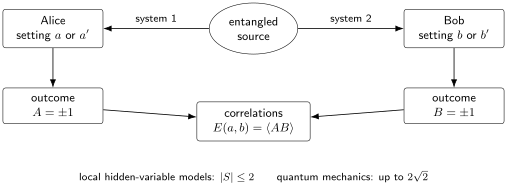
The CHSH data object is assembled from four setting subensembles. The shared source can correlate the outcomes, but the Bell-local model restricts each response to its local setting and the shared variable. The diagram records the local bound and the quantum ceiling; the algebraic no-signaling ceiling is $4$.

The containments relevant to this scenario are

$$\text{Bell-local} \subsetneq \text{quantum} \subsetneq \text{no-signaling}.$$

The numerical bounds are witnesses of those strict containments; they should not be interpreted as three possible signal speeds.

What a CHSH violation establishes

If the analyzed data faithfully estimate $p(a,b\mid x,y)$, the settings are independent of the hidden variables, and the statistical evidence establishes $\lvert S\rvert>2$, then no Bell-local factorized model can reproduce those correlators. Within quantum mechanics, such a violation also certifies that the measured state was entangled.

It does not establish any of the following by itself:

• that controllable information traveled faster than light;
• that every hidden-variable theory is impossible;
• that all entangled states violate CHSH;
• that one particular interpretation of quantum mechanics is correct;
• that four outcomes existed as jointly observed facts on each trial;
• that finite-sample, detection, or setting-choice assumptions can be ignored.

The theorem is exact, but its application to an experiment requires a declared estimator, uncertainty analysis, setting-generation model, and trial-selection rule. Those empirical questions should not be folded silently into the algebraic inequality.

Common pitfalls

Using four outcomes from one trial. The four correlators are estimated on different setting subensembles. A deterministic four-entry response table is an extreme point of a local model, not a record of four simultaneous measurements.

Adding determinism as an unexplained premise. The stochastic derivation already gives the local bound. Deterministic strategies are sufficient because their convex mixtures generate the finite local set.

Calling $4$ the quantum maximum. Four is the algebraic and no-signaling maximum. Quantum observables obey the stronger Tsirelson bound $2\sqrt2$.

Inferring signaling from violation. The singlet distribution has uniform, remote-setting-independent marginals even at maximal quantum violation.

Equating entanglement with CHSH violation. Every CHSH-violating quantum state is entangled, but not every entangled mixed state violates CHSH.

Exercises

1. Deterministic strategies saturate the local bound

Let $A_0,A_1,B_0,B_1\in\{-1,+1\}$. Show directly that

$$A_0B_0+A_0B_1+A_1B_0-A_1B_1$$

is always $+2$ or $-2$.

Solution

Factor the expression as

$$A_0(B_0+B_1)+A_1(B_0-B_1).$$

If $B_0=B_1$, the second parenthesis vanishes and the first is $\pm2$. If $B_0=-B_1$, the first vanishes and the second is $\pm2$. Multiplication by $A_0$ or $A_1$ can change only the sign, not the magnitude.

2. Complete the stochastic inequality

Suppose $m_0,m_1,n_0,n_1\in[-1,1]$. Prove

$$\left\lvert m_0(n_0+n_1)+m_1(n_0-n_1) \right\rvert \leq2.$$

Solution

Using $\lvert m_0\rvert,\lvert m_1\rvert\leq1$ gives

$$\lvert s\rvert \leq \lvert n_0+n_1\rvert + \lvert n_0-n_1\rvert.$$

For real $u,v$,

$$\lvert u+v\rvert+\lvert u-v\rvert = 2\max(\lvert u\rvert,\lvert v\rvert).$$

Taking $u=n_0$ and $v=n_1$ makes the right-hand side at most $2$. Integration over any normalized hidden-variable distribution preserves the bound.

3. Check the singlet probabilities

For the optimal directions, compute the joint probabilities when $x=y=0$. Verify normalization, uniform marginals, and $E_{00}=1/\sqrt2$.

Solution

Here $\mathbf u_0\cdot\mathbf v_0=-1/\sqrt2$, so

$$p(a,b\mid0,0) = \frac14\left(1+\frac{ab}{\sqrt2}\right).$$

The equal-sign outcomes each have probability $\tfrac14(1+1/\sqrt2)$, and the unequal-sign outcomes each have probability $\tfrac14(1-1/\sqrt2)$. Their sum is one. Summing over either sign of the remote outcome gives $1/2$. Finally,

$$E_{00} = P(a=b)-P(a\ne b) = \frac1{\sqrt2}.$$

4. Find the white-noise threshold

The state $\rho_v$ has optimal CHSH value $2\sqrt2v$. Find the visibility at which it begins to violate the local bound, and evaluate the maximum at $v=0.70$.

Solution

Violation requires

$$2\sqrt2v>2,$$

so $v>1/\sqrt2\approx0.7071$. At $v=0.70$,

$$S_{\max}=1.4\sqrt2\approx1.980,$$

which does not violate CHSH even though $v>1/3$ and the state is entangled.

5. Audit the PR box

Verify that the PR distribution is normalized and no-signaling, compute its four sign correlators, and identify which two bounds it exceeds or saturates.

Solution

For each $x,y$, exactly two output pairs satisfy $r\mathbin{\oplus}s=xy$, each with probability $1/2$, so the distribution is normalized. For any fixed local output there is exactly one compatible remote output, giving both marginals $1/2$ independently of the remote setting.

Mapping to signs gives $ab=(-1)^{xy}$, hence

$$E_{00}=E_{01}=E_{10}=1, \qquad E_{11}=-1.$$

Therefore $S=4$. The box exceeds both the Bell-local bound $2$ and the quantum bound $2\sqrt2$, while saturating the algebraic and no-signaling maximum $4$.

References

• J. S. Bell, “On the Einstein Podolsky Rosen Paradox,” Physics Physique Fizika 1, 195–200, 1964, doi:10.1103/PhysicsPhysiqueFizika.1.195.
• N. Brunner, D. Cavalcanti, S. Pironio, V. Scarani, and S. Wehner, “Bell Nonlocality,” Reviews of Modern Physics 86, 419–478, 2014, doi:10.1103/RevModPhys.86.419.
• B. S. Cirel’son, “Quantum Generalizations of Bell’s Inequality,” Letters in Mathematical Physics 4, 93–100, 1980, doi:10.1007/BF00417500.
• J. F. Clauser, M. A. Horne, A. Shimony, and R. A. Holt, “Proposed Experiment to Test Local Hidden-Variable Theories,” Physical Review Letters 23, 880–884, 1969, doi:10.1103/PhysRevLett.23.880.
• A. Fine, “Hidden Variables, Joint Probability, and the Bell Inequalities,” Physical Review Letters 48, 291–295, 1982, doi:10.1103/PhysRevLett.48.291.
• R. Horodecki, P. Horodecki, and M. Horodecki, “Violating Bell Inequality by Mixed Spin-1/2 States: Necessary and Sufficient Condition,” Physics Letters A 200, 340–344, 1995, doi:10.1016/0375-9601(95)00214-N.
• S. Popescu and D. Rohrlich, “Quantum Nonlocality as an Axiom,” Foundations of Physics 24, 379–385, 1994, doi:10.1007/BF02058098.
• R. F. Werner, “Quantum States with Einstein-Podolsky-Rosen Correlations Admitting a Hidden-Variable Model,” Physical Review A 40, 4277–4281, 1989, doi:10.1103/PhysRevA.40.4277.