Concept Map

This page is a map of the whole volume. It is meant for orientation: start at the tensor-product rule, then follow the branches toward product states, local observables, reduced states, entanglement diagnostics, identical-particle sectors, Fock space, and second quantization.

It does not own the derivations. Use the links in each section for canonical explanations.

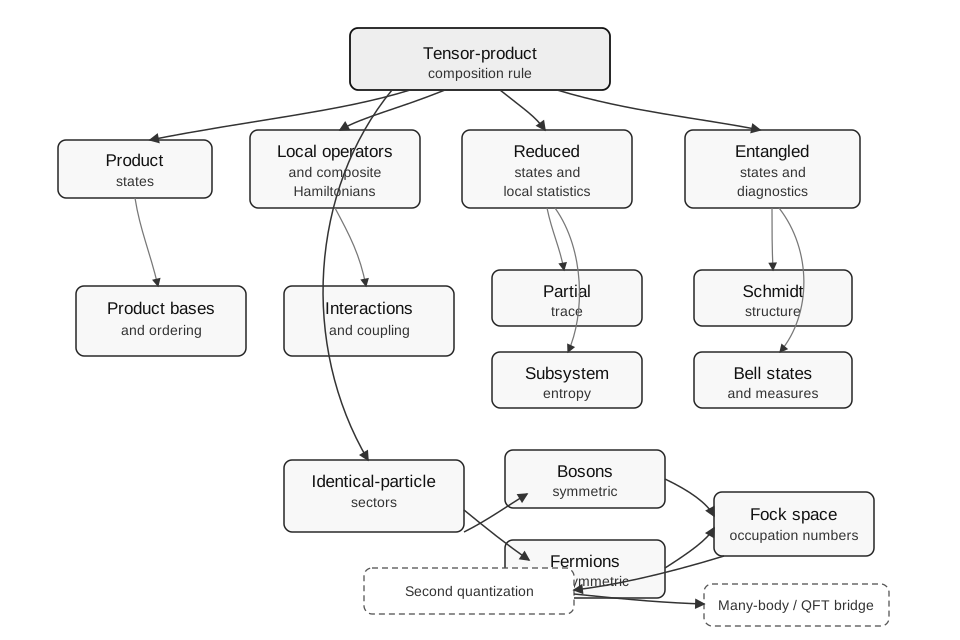
Concept map for the volume. The tensor product $\mathcal H_A\otimes\mathcal H_B$ organizes distinguishable subsystems; identical particles require symmetric or antisymmetric sectors and lead naturally to Fock space and second quantization.

How to Read the Map

The central rule is

$$\mathcal H_{AB} = \mathcal H_A\otimes\mathcal H_B.$$

For distinguishable subsystems, this rule tells us how state spaces combine. From it come product states, product bases, local operators, composite Hamiltonians, and the possibility of entanglement.

The main caution is that “composite” does not mean “entangled.” A composite Hilbert space contains product states and entangled states. Entanglement is a special property of a state relative to a specified subsystem decomposition.

Product and Local Structure

The first branch is the product side of the map. A pure product state has the form

$$\lvert\Psi\rangle = \lvert\psi\rangle_A\otimes\lvert\phi\rangle_B.$$

It has no correlation between $A$ and $B$. Product states are the baseline against which separability, entanglement, and correlations are defined.

Local operators are embedded by adding identity factors:

$$O_A \mapsto O_A\otimes I_B, \qquad O_B \mapsto I_A\otimes O_B.$$

This notation is not cosmetic. It fixes which subsystem an operator acts on and how the operator is represented as a matrix in a product basis. The canonical pages are Product Bases and Operators on Composite Systems.

Hamiltonians and Couplings

A noninteracting bipartite Hamiltonian has the form

$$H_0 = H_A\otimes I_B + I_A\otimes H_B.$$

Interactions add terms that do not belong to either subsystem alone:

$$H = H_0+V_{AB}.$$

The interaction branch is where product states can become entangled under time evolution. It is also where composite quantum mechanics connects to atoms, molecules, spin chains, detectors, and effective models. Later pages in this volume treat composite Hamiltonians and coupling terms more directly; until then, Why Composite Systems Matter gives the motivation.

Reduced States

The reduced-state branch asks what a subsystem can predict on its own. Given a joint density operator $\rho_{AB}$,

$$\rho_A = \operatorname{Tr}_B\rho_{AB}$$

is the state that reproduces all local statistics on subsystem $A$.

The partial trace is not a projection, and it is not a measurement outcome. It discards the degrees of freedom of $B$ while keeping the statistics of $A$. This operation is the bridge from joint states to local measurements, subsystem entropy, purification, and open-system language.

The canonical route is:

• Reduced Density Operators
• Partial Trace
• Local Measurement Statistics
• Subsystem Entropy

Entanglement Branch

The entanglement branch starts with the failure of product form. For a pure bipartite state,

$$\lvert\Psi\rangle \ne \lvert\psi\rangle_A\otimes\lvert\phi\rangle_B$$

for every choice of local vectors. Such a state is entangled across $A\vert B$.

For finite-dimensional pure states, the Schmidt decomposition gives the cleanest diagnostic:

$$\lvert\Psi\rangle = \sum_{r=1}^{R} s_r \lvert r_A\rangle \lvert r_B\rangle.$$

The state is product if $R=1$ and entangled if $R>1$. The same Schmidt coefficients determine the pure-state entanglement entropy.

For mixed states, one needs different tools: separability, PPT tests, concurrence in the two-qubit case, negativity, and entanglement witnesses. The Entanglement Diagnostic Table summarizes which diagnostic applies in which setting.

Identical Particles

The identical-particle branch changes the meaning of “subsystem.” If the particles are indistinguishable, labels such as particle $1$ and particle $2$ are not physical names of trackable individuals. The state space is constrained:

$$\Psi(x_1,x_2) = \Psi(x_2,x_1) \quad \text{for bosons},$$

and

$$\Psi(x_1,x_2) = - \Psi(x_2,x_1) \quad \text{for fermions}.$$

Bosons live in symmetric sectors; fermions live in antisymmetric sectors. This is the conceptual path to Bose enhancement, Pauli exclusion, Slater determinants, permanents, and occupation-number notation.

Start with Indistinguishability and Symmetrization Postulate, then continue to Bosons or Fermions.

Fock Space and Second Quantization

Fock space appears when particle number is allowed to vary or when mode occupation is the cleanest language:

$$\mathcal F = \mathcal H_0\oplus\mathcal H_1\oplus\mathcal H_2\oplus\cdots.$$

For bosons and fermions, the $N$-particle sectors are symmetric or antisymmetric. Occupation-number states then replace labeled-particle wavefunctions as the practical basis:

$$\lvert n_1,n_2,\ldots\rangle.$$

Creation and annihilation operators change occupations. This is the bridge to many-body Hamiltonians, quantum optics, quantum chemistry, condensed matter, and eventually QFT.

The recommended route is:

• Occupation-Number Basis
• Bosonic Fock Space
• Fermionic Fock Space
• Creation and Annihilation Operators
• Second Quantization: Bridge to QFT

Decision Guide

Use the map as a routing tool:

• If the question asks how systems combine, start with Tensor Products of Hilbert Spaces.
• If the question asks how basis labels become arrays, use Product Bases and Notation and Subsystem Labels.
• If the question asks what subsystem $A$ can predict by itself, use Partial Trace.
• If the question asks whether a state is entangled, use Entangled States and then the Entanglement Diagnostic Table.
• If the question involves identical particles, start with Indistinguishability before applying ordinary tensor-factor intuition.
• If the question uses modes, occupation numbers, or creation operators, move to Fock Space Examples and the second-quantization pages.

Common Mistakes

• Treating the tensor product as only a notation for putting two vectors side by side.
• Jumping from “state is composite” to “state is entangled.”
• Using partial trace as though it were a postselected measurement.
• Applying distinguishable-particle subsystem language to identical particles without specifying modes or regions.
• Starting second quantization before the occupation-number basis is clear.
• Looking for one universal entanglement diagnostic that works for pure, mixed, many-body, Gaussian, and identical-particle settings without assumptions.

Cross-Links

• Composite Systems and Entanglement
• Why Composite Systems Matter
• Notation and Subsystem Labels
• Tensor Products of Hilbert Spaces
• Product States
• Entangled States
• Partial Trace
• Schmidt Decomposition
• Identical-Particle Entanglement Cautions
• Fock Space Examples
• Formula Sheet
• Common Composite States
• Entanglement Diagnostic Table

References

• P. A. M. Dirac, The Principles of Quantum Mechanics, 4th ed., Oxford University Press, 1958.
• E. Schrodinger, “Discussion of Probability Relations between Separated Systems,” Mathematical Proceedings of the Cambridge Philosophical Society 31, 555-563, 1935.
• R. Shankar, Principles of Quantum Mechanics, 2nd ed., Springer, 1994.
• J. J. Sakurai and J. Napolitano, Modern Quantum Mechanics, 3rd ed., Cambridge University Press, 2020.
• M. A. Nielsen and I. L. Chuang, Quantum Computation and Quantum Information, Cambridge University Press, 2010.
• A. L. Fetter and J. D. Walecka, Quantum Theory of Many-Particle Systems, McGraw-Hill, 1971.

Exercises

1. Route through the map. A two-qubit pure state has reduced density matrix $\rho_A=I/2$. Which branch of the map explains the reduced state, and which branch decides whether the state is entangled?

Solution

The reduced-state branch explains how $\rho_A$ is obtained: compute $\rho_A=\operatorname{Tr}_B\rho_{AB}$. The entanglement branch decides whether the pure state is entangled. For a pure bipartite state, $\rho_A=I/2$ is mixed, so the state is entangled across the two-qubit split.

2. Identical-particle routing. Two electrons are described by an antisymmetric wavefunction. Which branch should be consulted before calling the state entangled?

Solution

Use the identical-particle branch first. Antisymmetry is a constraint on fermionic states, not automatically an ordinary entanglement resource between labeled particles. One must specify a physical split, such as modes, spin-orbitals, spatial regions, or accessible observables, before applying entanglement language.

3. Fock-space routing. A calculation uses states $\lvert n_1,n_2,\ldots\rangle$ and operators $a_i^\dagger,a_i$. Which part of the map is active?

Solution

This is the Fock-space and second-quantization branch. The states are occupation-number states, and $a_i^\dagger,a_i$ are creation and annihilation operators for modes. The relevant canonical pages are the occupation-number basis, bosonic or fermionic Fock space, and creation-annihilation operators.