Dirac to Pauli

The Pauli Hamiltonian is not obtained by merely deleting the lower two components of a Dirac spinor. In the Dirac basis, those components are small in a positive-energy, low-momentum regime, but they mediate the magnetic spin coupling. Solving for them to leading order gives

$$H_{\mathrm{eff}} = q\Phi +\frac{\boldsymbol\pi^2}{2m} -\frac{q\hbar}{2m} \boldsymbol\sigma\cdot\mathbf B,$$

where $q$ is signed and $\boldsymbol\pi=-i\hbar\nabla-q\mathbf A$. The coefficient corresponds to the tree-level Dirac value $g=2$. This page derives that result and states the hierarchy needed to trust it.

Required background. The Covariant Dirac Equation, Gamma-Matrix Conventions, and Minimal Coupling supply the Hamiltonian, Dirac basis, signed charge, and kinetic-momentum commutator. Two-component Pauli algebra and controlled asymptotic expansions are assumed.

Separate the rest energy and spinor blocks

The minimally coupled Dirac equation in Hamiltonian form is

$$i\hbar\partial_t\psi = \left( c\boldsymbol\alpha\cdot\boldsymbol\pi +\beta mc^2 +q\Phi \right)\psi.$$

In the Dirac basis,

$$\boldsymbol\alpha\cdot\boldsymbol\pi = \begin{pmatrix} 0_2&\boldsymbol\sigma\cdot\boldsymbol\pi\\ \boldsymbol\sigma\cdot\boldsymbol\pi&0_2 \end{pmatrix}, \qquad \beta = \begin{pmatrix} I_2&0_2\\ 0_2&-I_2 \end{pmatrix}.$$

For a state concentrated in the positive-energy sector, remove the rest- energy phase and write

$$\psi(t,\mathbf x) = e^{-imc^2t/\hbar} \begin{pmatrix} \varphi(t,\mathbf x)\\ \chi(t,\mathbf x) \end{pmatrix}.$$

The two-component amplitudes $\varphi$ and $\chi$ are often called the large and small components in this regime. Those names are conclusions of the scale hierarchy, not permanent basis-independent labels.

Substitution gives the exact coupled equations

$$i\hbar\partial_t\varphi = q\Phi\varphi +c\boldsymbol\sigma\cdot\boldsymbol\pi\,\chi,$$

and

$$i\hbar\partial_t\chi = c\boldsymbol\sigma\cdot\boldsymbol\pi\,\varphi +(q\Phi-2mc^2)\chi.$$

The lower block lies a rest-energy gap $2mc^2$ away after the positive-branch phase has been removed. Losing this factor of two gives the wrong magnetic and kinetic coefficients.

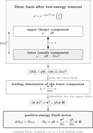
After removing $mc^2$, the upper component is slow while the lower component is offset by $-2mc^2$. The off-diagonal operator $c\boldsymbol\sigma\cdot\boldsymbol\pi$ creates the leading small component; substituting it back produces both kinetic and magnetic terms.

Leading elimination of the small component

Rearrange the lower equation:

$$\left( 2mc^2+i\hbar\partial_t-q\Phi \right)\chi = c\boldsymbol\sigma\cdot\boldsymbol\pi\,\varphi.$$

The positive-energy nonrelativistic regime requires gauge-covariant residual energies and kinetic couplings small compared with the gap. An absolute scalar-potential offset is gauge dependent; physically relevant potential differences and transition frequencies must respect the expansion. A useful local hierarchy is

$$\left|i\hbar\partial_t-q\Phi\right| \ll2mc^2, \qquad c|\boldsymbol\pi|\ll2mc^2,$$

together with fields that vary slowly enough not to induce transitions across the gap. To leading order, replace the operator in parentheses by $2mc^2$:

$$\chi \simeq \frac{\boldsymbol\sigma\cdot\boldsymbol\pi}{2mc}\,\varphi.$$

For a free positive-energy packet, this estimates

$$\frac{\|\chi\|}{\|\varphi\|} \sim \frac{|\mathbf p|}{2mc} \sim \frac{v}{2c}.$$

Setting $\chi=0$ would discard the entire order needed to generate the Pauli spin term. The correct leading procedure is to solve for $\chi$ and substitute it into the upper equation.

For spatially or temporally varying potentials, the formal inverse

$$\chi = \left( 2mc^2+i\hbar\partial_t-q\Phi \right)^{-1} c\boldsymbol\sigma\cdot\boldsymbol\pi\,\varphi$$

is an ordered operator expression. Expanding it beyond leading order requires care with noncommuting time derivatives, potentials, and kinetic momenta.

The Pauli identity with noncommuting momenta

Use

$$\sigma_i\sigma_j = \delta_{ij}I_2+i\epsilon_{ijk}\sigma_k.$$

Then

$$\begin{aligned} (\boldsymbol\sigma\cdot\boldsymbol\pi)^2 &= \sigma_i\sigma_j\pi_i\pi_j \\ &= \boldsymbol\pi^2 +i\epsilon_{ijk}\sigma_k\pi_i\pi_j \\ &= \boldsymbol\pi^2 +\frac{i}{2}\epsilon_{ijk}\sigma_k[\pi_i,\pi_j]. \end{aligned}$$

Minimal coupling gives

$$[\pi_i,\pi_j] = iq\hbar\epsilon_{ij\ell}B_\ell.$$

Using $\epsilon_{ijk}\epsilon_{ij\ell}=2\delta_{k\ell}$,

$$\boxed{ (\boldsymbol\sigma\cdot\boldsymbol\pi)^2 = \boldsymbol\pi^2 -q\hbar\boldsymbol\sigma\cdot\mathbf B }.$$

The magnetic term is a direct consequence of the noncommuting kinetic momenta. If one replaces $\pi_i\pi_j$ by commuting numbers, the spin coupling vanishes incorrectly.

Effective Pauli Hamiltonian

Substitute the leading $\chi$ into the upper equation:

$$i\hbar\partial_t\varphi = q\Phi\varphi +\frac{1}{2m} (\boldsymbol\sigma\cdot\boldsymbol\pi)^2\varphi.$$

The Pauli identity gives

$$i\hbar\partial_t\varphi = \left[ q\Phi +\frac{\boldsymbol\pi^2}{2m} -\frac{q\hbar}{2m} \boldsymbol\sigma\cdot\mathbf B \right]\varphi.$$

With the physical spin operator

$$\mathbf S=\frac{\hbar}{2}\boldsymbol\sigma,$$

the magnetic term is

$$-\frac{q}{m}\mathbf S\cdot\mathbf B = -g\frac{q}{2m}\mathbf S\cdot\mathbf B \quad\text{with}\quad g=2.$$

For an electron, $q=-e$, so

$$-\frac{q\hbar}{2m}\boldsymbol\sigma\cdot\mathbf B = +\frac{e\hbar}{2m}\boldsymbol\sigma\cdot\mathbf B.$$

This sign says that an electron’s magnetic moment is antiparallel to its spin. The lower-energy Zeeman state in a positive $z$ field therefore has spin antiparallel to $\mathbf B$.

What this approximation has and has not done

The algebraic elimination above is a leading positive-energy approximation. It is not the full Foldy–Wouthuysen transformation. A systematic Foldy–Wouthuysen construction seeks a unitary block diagonalization of the Dirac Hamiltonian order by order, transforming states and observables as well as the Hamiltonian.

At higher order, a controlled calculation can generate:

• the free kinetic correction $-\mathbf p^4/(8m^3c^2)$;
• spin–orbit coupling;
• the Darwin term;
• field-gradient, time-dependence, and operator-ordering contributions.

Their exact form depends on assumptions such as static versus time-dependent fields, the retained field order, commutator ordering, and Hermitian symmetrization. Printing one compact “general” $O(c^{-2})$ Hamiltonian without those assumptions would overclaim. Those corrections therefore remain outside this leading-order result; any higher-order extension must declare its field, ordering, and block-diagonalization assumptions explicitly.

The Foldy–Wouthuysen Transformation owns the representation change and transformed observables. The static Foldy–Wouthuysen expansion provides those declared assumptions and derives the higher-order operators.

The leading Pauli result is reliable when the state stays far from the negative-energy sector, momenta are small compared with $mc$, external fields are weak and slowly varying on the Compton scale, and pair creation is negligible. It does not provide a Lorentz-covariant two-component theory or a description of antiparticles.

Common pitfalls

Deleting the small component. Although $\chi$ is suppressed, its leading value generates the kinetic and magnetic operators. Solve for it before truncating.

Using $mc^2$ instead of $2mc^2$. After the positive rest-energy phase is removed, the negative-energy block is separated by twice the rest energy.

Commuting the kinetic momenta. Their antisymmetric product contains $\mathbf B$ and is exactly what produces the spin term.

Calling the result exact. The Pauli Hamiltonian is the leading low-energy positive-sector theory. Relativistic, radiative, and pair-production effects remain outside it.

Exercises

1. Coupled component equations

Starting from the Dirac-basis Hamiltonian, reproduce both exact equations for $\varphi$ and $\chi$ after removing the rest-energy phase.

Solution

The left side contains an added $mc^2$ multiplying both components. On the right, $\beta mc^2$ contributes $+mc^2$ to the upper block and $-mc^2$ to the lower. Cancellation in the upper equation leaves

$$i\hbar\partial_t\varphi =q\Phi\varphi+c\boldsymbol\sigma\cdot\boldsymbol\pi\,\chi.$$

In the lower equation the two rest-energy contributions combine to $-2mc^2\chi$, giving

$$i\hbar\partial_t\chi =c\boldsymbol\sigma\cdot\boldsymbol\pi\,\varphi +(q\Phi-2mc^2)\chi.$$

2. Noncommuting Pauli identity

Derive $(\boldsymbol\sigma\cdot\boldsymbol\pi)^2$ without assuming that the components of $\boldsymbol\pi$ commute.

Solution

Only the antisymmetric part of $\pi_i\pi_j$ survives contraction with $\epsilon_{ijk}$:

$$i\epsilon_{ijk}\sigma_k\pi_i\pi_j = \frac{i}{2}\epsilon_{ijk}\sigma_k[\pi_i,\pi_j].$$

Substituting $[\pi_i,\pi_j]=iq\hbar\epsilon_{ij\ell}B_\ell$ and contracting the epsilon symbols gives $-q\hbar\boldsymbol\sigma\cdot\mathbf B$.

3. Electron sign

Set $q=-e$ with $e>0$ in the effective Hamiltonian. Which spin projection has lower energy in a uniform field $\mathbf B=B\hat{\mathbf z}$?

Solution

The spin term is

$$H_{\mathrm{spin}} = +\frac{e\hbar B}{2m}\sigma_z.$$

Its eigenvalues are $\pm e\hbar B/(2m)$. The $\sigma_z=-1$ state, whose spin is antiparallel to $\mathbf B$, has the lower energy.

4. Size of the small component

Estimate $\|\chi\|/\|\varphi\|$ for a free packet with speed $v=10^{-2}c$.

Solution

At leading order $|\mathbf p|\simeq mv$, so

$$\frac{\|\chi\|}{\|\varphi\|} \sim \frac{|\mathbf p|}{2mc} \simeq \frac{v}{2c} =5\times10^{-3}.$$

The probability weight of the lower component is smaller by roughly the square of this ratio.

References

• L. L. Foldy and S. A. Wouthuysen, “On the Dirac Theory of Spin 1/2 Particles and Its Non-Relativistic Limit,” Physical Review 78, 29–36, 1950, doi:10.1103/PhysRev.78.29.
• W. Greiner, Relativistic Quantum Mechanics: Wave Equations, 3rd ed., Springer, 2000, doi:10.1007/978-3-662-04275-5.
• J. J. Sakurai, Advanced Quantum Mechanics, Addison–Wesley, 1967.
• F. Schwabl, Advanced Quantum Mechanics, 3rd ed., Springer, 2005, doi:10.1007/3-540-28528-8.