Time Slicing

Time slicing is the finite-partition construction behind the path-integral symbol

$$\int \mathcal D x(t)\,e^{iS[x]/\hbar}.$$

The continuum notation is compact, but the real definition begins with a finite number of time steps, ordinary integrals over intermediate positions, and short-time kernels with normalization factors. Time slicing is where the measure, action discretization, and operator-ordering choices enter.

Discretizing Time

Fix endpoints

$$(x_i,t_i), \qquad (x_f,t_f),$$

and define

$$T=t_f-t_i.$$

Choose $N$ equal time steps

$$\epsilon=\frac{T}{N},$$

with

$$t_j=t_i+j\epsilon, \qquad j=0,1,\ldots,N.$$

The endpoint positions are fixed:

$$x_0=x_i, \qquad x_N=x_f.$$

The intermediate positions $x_1,\ldots,x_{N-1}$ are variables to be integrated over.

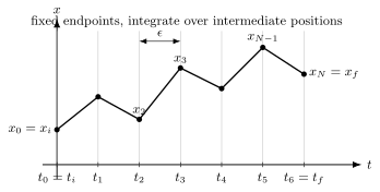
A path integral starts from a finite partition $t_j=t_i+j\epsilon$, fixed endpoints $x_0=x_i$ and $x_N=x_f$, and integrations over intermediate positions $x_1,\ldots,x_{N-1}$.

Intermediate Positions

The propagator kernel is

$$K(x_f,t_f;x_i,t_i) = \langle x_f|U(t_f,t_i)|x_i\rangle.$$

Use the composition law

$$U(t_f,t_i) = U(t_N,t_{N-1})\cdots U(t_1,t_0).$$

Between each short-time factor, insert the position resolution of identity:

$$I=\int_{-\infty}^{\infty}dx_j\,|x_j\rangle\langle x_j|.$$

This gives

$$\begin{aligned} K(x_f,t_f;x_i,t_i) &= \int dx_1\cdots dx_{N-1} \\ &\quad \times \prod_{j=0}^{N-1} K_\epsilon(x_{j+1},x_j;t_j), \end{aligned}$$

where

$$K_\epsilon(x_{j+1},x_j;t_j) = \langle x_{j+1}|U(t_{j+1},t_j)|x_j\rangle.$$

The product order follows time order: earlier factors act first and appear to the right in the operator product.

Short-Time Kernel

For

$$H=\frac{p^2}{2m}+V(x),$$

one uses a short-time approximation to

$$U(t_{j+1},t_j) = e^{-iH\epsilon/\hbar}.$$

A first-order kinetic-potential splitting gives

$$e^{-iH\epsilon/\hbar} = e^{-ip^2\epsilon/(2m\hbar)} e^{-iV(x)\epsilon/\hbar} +O(\epsilon^2)$$

in operator norm for sufficiently controlled bounded models, and formally for many standard unbounded wave-mechanics models. In coordinate representation this leads to

$$\begin{aligned} K_\epsilon(x_{j+1},x_j) &\approx \left( \frac{m}{2\pi i\hbar\epsilon} \right)^{1/2} \\ &\quad \times \exp\left\{ \frac{i}{\hbar}\epsilon \left[ \frac{m}{2} \left( \frac{x_{j+1}-x_j}{\epsilon} \right)^2 -V(x_j) \right] \right\}. \end{aligned}$$

The kinetic factor is the free-particle short-time kernel. The potential factor is diagonal in position space.

Trotter Product Relation

The short-time splitting is a Trotter product formula in disguise. If

$$T_p=\frac{p^2}{2m},$$

then

$$e^{-i(T_p+V)\epsilon/\hbar} \approx e^{-iT_p\epsilon/\hbar} e^{-iV\epsilon/\hbar}.$$

A symmetric second-order step is

$$e^{-iH\epsilon/\hbar} \approx e^{-iV\epsilon/(2\hbar)} e^{-iT_p\epsilon/\hbar} e^{-iV\epsilon/(2\hbar)}.$$

This corresponds to evaluating the potential more symmetrically along each time slice. In the continuum limit, different discretizations can agree for simple Hamiltonians, but in more complicated systems they may encode different operator orderings. The details are not cosmetic.

Discretized Action

Using the first-order short-time kernel, the product over slices gives

$$K(x_f,t_f;x_i,t_i) = \lim_{N\to\infty} \left( \frac{m}{2\pi i\hbar\epsilon} \right)^{N/2} \int dx_1\cdots dx_{N-1}\, e^{iS_N/\hbar},$$

where

$$S_N = \sum_{j=0}^{N-1} \epsilon \left[ \frac{m}{2} \left( \frac{x_{j+1}-x_j}{\epsilon} \right)^2 -V(x_j) \right].$$

The expression $S_N$ is the discretized action. The formal continuum statement

$$S_N\to \int_{t_i}^{t_f}dt\, \left[ \frac{m}{2}\dot x^2-V(x) \right]$$

is a mnemonic for this limiting construction, not a license to forget the discretization.

Measure Factors

The path-integral measure symbol hides the finite-dimensional normalization:

$$\int\mathcal D x(t) \quad\text{means schematically}\quad \lim_{N\to\infty} \left( \frac{m}{2\pi i\hbar\epsilon} \right)^{N/2} \prod_{j=1}^{N-1} \int dx_j.$$

This factor has dimensions. For one coordinate, each short-time kernel has dimension $1/\text{length}$, and after $N-1$ intermediate integrations the full kernel still has dimension $1/\text{length}$. Dropping the normalization changes the amplitude, not just an irrelevant convention.

For multidimensional systems, constrained systems, curved configuration spaces, fields, or fermions, the measure changes. Propagators in Multiple Dimensions gives the flat-space $d$-coordinate formula and explains why coordinate Jacobians, kinetic operators, and short-time factors must be transformed together.

Continuum Notation

The continuum notation

$$K(x_f,t_f;x_i,t_i) = \int_{x(t_i)=x_i}^{x(t_f)=x_f} \mathcal D x(t)\, e^{iS[x]/\hbar}$$

is useful because it displays the physical structure: amplitudes are weighted by the action phase and summed over histories. But the notation suppresses:

• the time partition;
• normalization factors;
• endpoint conditions;
• the choice of where each potential is evaluated;
• operator-ordering conventions;
• convergence or regularization prescriptions.

In real time, the weight $e^{iS/\hbar}$ is oscillatory. It is not a probability measure on paths.

Common Normalization Mistakes

• Writing only $e^{iS_N/\hbar}$ and dropping the product of short-time prefactors.
• Integrating over the endpoints even though the propagator fixes them.
• Forgetting that $N$ short-time kernels give $N$ prefactors but only $N-1$ intermediate position integrals.
• Treating $\mathcal D x$ as if it were an ordinary translation-invariant measure on a space of smooth functions.
• Changing Fourier-transform conventions without updating the short-time prefactor.
• Assuming a midpoint rule, left-endpoint rule, and right-endpoint rule always define the same quantum operator.

Cross-Links

• From Propagators to Path Integrals
• Why Path Integrals?
• Action and Phase
• Stationary Phase and the Classical Limit
• Path Integral Conventions
• Common Pitfalls in Path Integrals
• Trotter Product Formula
• Free-Particle Propagator
• Propagators in Multiple Dimensions
• Action Principles
• Functional Derivatives
• QFT Bridge: Path Integrals

References

• R. P. Feynman and A. R. Hibbs, Quantum Mechanics and Path Integrals, McGraw-Hill, 1965.
• L. S. Schulman, Techniques and Applications of Path Integration, Wiley, 1981.
• H. Kleinert, Path Integrals in Quantum Mechanics, Statistics, Polymer Physics, and Financial Markets, 5th ed., World Scientific, 2009.
• J. Zinn-Justin, Path Integrals in Quantum Mechanics, Oxford University Press, 2005.
• M. Chaichian and A. Demichev, Path Integrals in Physics, Volume I, Institute of Physics Publishing, 2001.

Exercises

1. For $N$ time intervals, why are there $N-1$ intermediate position integrations?

Solution

The positions $x_0=x_i$ and $x_N=x_f$ are fixed by the propagator endpoints. The remaining positions $x_1,\ldots,x_{N-1}$ are not fixed, so each is integrated over. There are $N-1$ such intermediate variables.

2. Check the dimension of the one-dimensional free short-time prefactor.

Solution

The combination $\hbar\epsilon/m$ has dimensions of length squared:

$$\frac{\hbar\epsilon}{m} \sim \frac{ML^2T^{-1}\,T}{M} = L^2.$$

Therefore

$$\left( \frac{m}{2\pi i\hbar\epsilon} \right)^{1/2}$$

has dimension $1/L$, as a coordinate-space kernel should in one dimension.

3. Show that the discretized kinetic term equals $m(x_{j+1}-x_j)^2/(2\epsilon)$ on each slice.

Solution

The finite-difference velocity on the slice is

$$\dot x_j \approx \frac{x_{j+1}-x_j}{\epsilon}.$$

The kinetic contribution to the action is

$$\epsilon\,\frac{m}{2}\dot x_j^2 = \epsilon\,\frac{m}{2} \left( \frac{x_{j+1}-x_j}{\epsilon} \right)^2 = \frac{m(x_{j+1}-x_j)^2}{2\epsilon}.$$

4. In the first-order discretization above, why does $V(x_j)$ appear rather than an average over the whole slice?

Solution

The displayed short-time kernel used a left-endpoint splitting,

$$e^{-iH\epsilon/\hbar} \approx e^{-iT_p\epsilon/\hbar} e^{-iV(x)\epsilon/\hbar}.$$

Since $V(x)$ acts on the ket $|x_j\rangle$, the potential factor contributes $e^{-iV(x_j)\epsilon/\hbar}$. A symmetric Trotter splitting would lead to a different finite-slice convention, often associated with midpoint-like rules. The continuum limit can agree for simple Hamiltonians, but the discretization records the operator ordering.