Landau–Zener Simulation

The infinite-sweep Landau–Zener formula is exact, but a numerical propagation never begins at $x=-\infty$, never ends at $x=+\infty$, and never uses an infinitesimal step. This notebook turns those three differences into separate tests. It propagates a swept two-level state with a unitary fourth-order Magnus method, compares two independent integrators, varies the endpoint and step independently, and records both probability and phase-sensitive state error.

The main numerical result is intentionally less tidy than a single agreement number. With exact instantaneous eigenstates prepared and measured at finite endpoints, the transition probability approaches $e^{-2\pi\gamma}$ with an oscillatory error. At $\gamma=0.25$, the absolute error falls from $4.21\times10^{-4}$ at $X=4$ to $1.37\times10^{-6}$ at $X=64$, but it does not decrease monotonically between those windows. A calculation that instead prepares and measures the bare diabatic state can differ by more than one percentage point even at $X=64$.

Meanwhile, the production Magnus state at $\gamma=0.5$ and $X=12$ changes by only $7.59\times10^{-13}$ when the step is halved. The residual difference from the asymptotic formula is therefore an endpoint effect, not an integration error.

Run the investigation. Download the complete package, extract it, and run python run.py --output-dir results in the environment described by Running an Experiment. The package verification report records the tested source, actual execution date, environment and scientific checks.

Canonical Boundaries

This page owns a reusable numerical experiment, not the general derivation of Landau–Zener physics.

Object	Canonical home	Role here
Hamiltonian, basis dictionary, and exact probability	Landau–Zener Transition	analytic target
convention audit and one hand-worked finite-window calculation	Landau–Zener Transition Worked Example	interpretation and comparison
general adiabatic criterion	Adiabatic Approximation	slow-passage context
convergence logic	Convergence Tests	numerical standard
reusable solver, sweeps, and retained data	this page	computational benchmark

The convention-sensitive state mapping is summarized here only to define the program’s input and output. Use the worked example when the factors of two or the words “stay” and “transition” are in doubt.

Physical Problem and Analytic Target

The Hamiltonian is

$$\begin{aligned} H(t) &= \frac{vt}{2}\sigma_z + \Delta\sigma_x, \\ v&>0, \qquad \Delta>0. \end{aligned}$$

Define

$$x \equiv \frac{vt}{2\Delta}, \qquad \gamma \equiv \frac{\Delta^2}{\hbar v}.$$

The time-dependent Schrödinger equation then becomes

$$i\frac{d\psi}{dx} = 2\gamma \left( x\sigma_z+\sigma_x \right)\psi.$$

The ideal infinite-sweep experiment prepares the lower instantaneous eigenstate at $x\to-\infty$ and asks for the probability of ending on the upper instantaneous branch at $x\to+\infty$. Its exact target is

$$P_{\mathrm{LZ}}(\gamma) = e^{-2\pi\gamma}.$$

Small $\gamma$ is the fast, nearly diabatic limit; large $\gamma$ is the slow, nearly adiabatic limit. The calculation below covers

$$0.02\le\gamma\le1.25,$$

for which the exact probability ranges from approximately $0.882$ to $3.88\times10^{-4}$.

Define the Finite Numerical Experiment

At a finite endpoint $X$, let $\lvert\pm;x\rangle$ denote normalized instantaneous eigenstates. The primary observable is

$$P_X = \left| \left\langle +;X\right| U(X,-X) \left|-;-X\right\rangle \right|^2.$$

This protocol prepares the exact lower eigenstate of the Hamiltonian actually used at the initial endpoint and projects onto the exact upper eigenstate at the final endpoint. Its difference from the asymptotic formula is

$$\epsilon_X = P_X-P_{\mathrm{LZ}}.$$

The program also evaluates a deliberately different protocol,

$$\widetilde P_X = \left| \langle1|U(X,-X)|1\rangle \right|^2,$$

where $\lvert1\rangle$ is a fixed diabatic basis vector. The two protocols agree only asymptotically. At finite $X$, replacing $\lvert-;-X\rangle$ by $\lvert1\rangle$ changes the preparation, and replacing $\lvert+;X\rangle$ by $\lvert1\rangle$ changes the measurement.

That distinction is not a small implementation detail. It is a change of physical question.

Numerical Propagators

Write the equation as

$$\begin{aligned} \frac{d\psi}{dx} &= A(x)\psi, \\ A(x) &= -2i\gamma \left( x\sigma_z+\sigma_x \right). \end{aligned}$$

Because $A(x)$ is anti-Hermitian, exact evolution is unitary. A time step should preserve that structure when practical.

Fourth-order Gauss–Magnus method

For a step from $x$ to $x+h$, define the midpoint $x_m=x+h/2$ and the two Gauss nodes

$$x_{1,2} = x_m \mp \frac{\sqrt3}{6}h.$$

With $A_j=A(x_j)$, the fourth-order Magnus exponent is

$$\Omega_4 = \frac{h}{2} \left(A_1+A_2\right) - \frac{\sqrt3h^2}{12} \left[A_1,A_2\right].$$

For the linear Landau–Zener Hamiltonian, the commutator can be evaluated analytically. The result is

$$\Omega_4=-iK,$$

with

$$\begin{aligned} K ={}& 2\gamma h\,\sigma_x + \frac{2}{3}\gamma^2h^3\,\sigma_y \\ &+ 2\gamma h x_m\,\sigma_z. \end{aligned}$$

If

$$\begin{aligned} K &= k_x\sigma_x+k_y\sigma_y+k_z\sigma_z, \\ r &= \sqrt{k_x^2+k_y^2+k_z^2}. \end{aligned}$$

then the step is applied without a general matrix exponential:

$$e^{-iK} = \cos r\,I - i\frac{\sin r}{r}K.$$

Each step is unitary to floating-point roundoff. The commutator term is essential for fourth-order accuracy; dropping it gives exponential midpoint.

Independent comparators

The program implements two additional methods.

1. Exponential midpoint: exponentiate $hA(x_m)$ exactly. It is unitary but only second order globally.
2. Classical RK4: evaluate four right-hand-side stages. It is fourth order in the asymptotic step-size regime but is neither exactly unitary nor unconditionally stable.

Agreement between Magnus and RK4 after refinement is stronger evidence than agreement between two nearly identical exponential formulas. Midpoint supplies a separate order check and demonstrates that exact norm preservation does not imply high accuracy.

Error Metrics

Probability error

At fixed $X$, the numerical probability is compared with a much finer Magnus reference:

$$\epsilon_P(h) = \left|P_h-P_{\mathrm{ref}}\right|.$$

A probability discards phase information. Its error can therefore be accidentally small even when the propagated state is not comparably accurate.

Phase-aligned state error

The primary integrator metric is

$$\epsilon_\psi(h) = \min_{\phi} \left\| \psi_h-e^{i\phi}\psi_{\mathrm{ref}} \right\|_2.$$

Removing one global phase compares physical rays while retaining relative amplitude and relative-phase errors. Both states are normalized before this comparison, so RK4 norm loss is also reported separately rather than hidden inside the distance.

Norm drift

The run records

$$\epsilon_N = \max_{-X\le x\le X} \left| \langle\psi(x)|\psi(x)\rangle-1 \right|.$$

For a unitary method, $\epsilon_N$ should remain near accumulated roundoff. For RK4 it is a stability and truncation diagnostic, but a small norm drift alone does not certify the state.

Production Parameters

Control	Production value	Independent sweep or check
endpoint for formula comparison	$X=64$	$4$ through $64$
step	$h=0.0025$	$0.16$ through $0.0025$
production method	fourth-order Magnus	midpoint and RK4
coupling	$0.02\le\gamma\le1.25$	nine retained values
trajectory example	$\gamma=0.25$, $X=12$	$801$ output samples
finite-step reference	Magnus, $h=0.0003125$	fixed $\gamma=0.5$, $X=12$
arithmetic	IEEE 754 binary64	norm and refinement audit
random sampling	none	deterministic output

At the largest endpoint and coupling, the instantaneous generator has eigenvalue magnitude

$$2\gamma\sqrt{1+X^2} \approx160.$$

Thus the endpoint dynamics, not only the central avoided crossing, constrain the step size. The production value gives a largest local phase increment of approximately $0.40$ for this hardest retained point.

Dynamics and Endpoint Convergence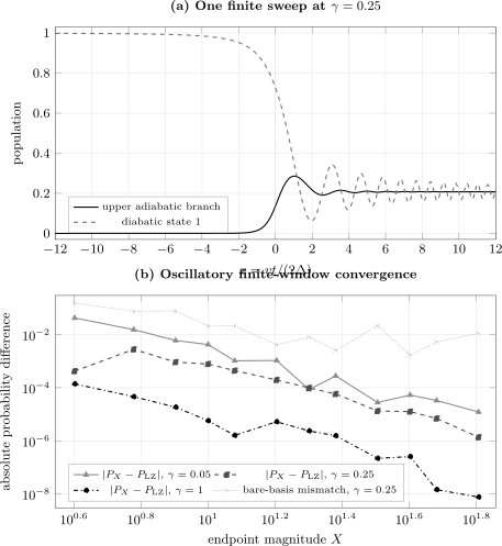

Panel (a) follows a state prepared as $\lvert-;-12\rangle$ at $\gamma=0.25$. The upper-adiabatic and first-diabatic populations answer different questions at finite $x$. Panel (b) shows the oscillatory difference $|P_X-P_{\mathrm{LZ}}|$ and, for $\gamma=0.25$, the difference between exact finite-endpoint and bare-diabatic protocols. A favorable single window is not a convergence proof.

The trajectory begins with unit lower-adiabatic population, but the same state already has diabatic population

$$|\langle1|-;-12\rangle|^2 = 0.998273.$$

At the crossing, the upper-adiabatic population is $0.136796$. At $x=12$ it is $0.2074385$, while the diabatic-$1$ population of that same propagated state is $0.2196466$. Neither finite-time quantity is required to equal the asymptotic result exactly.

One window sweep in detail

For $\gamma=0.25$,

$$P_{\mathrm{LZ}} = 0.2078795764.$$

| $X$ | $P_X$ | $P_X-P_{\mathrm{LZ}}$ | $|\widetilde P_X-P_X|$ | |---:|---:|---:|---:| | $4$ | $0.2074582473$ | $-4.21\times10^{-4}$ | $1.54\times10^{-1}$ | | $6$ | $0.2106734169$ | $+2.79\times10^{-3}$ | $7.59\times10^{-2}$ | | $8$ | $0.2088009714$ | $+9.21\times10^{-4}$ | $7.78\times10^{-2}$ | | $12$ | $0.2074385222$ | $-4.41\times10^{-4}$ | $2.15\times10^{-2}$ | | $16$ | $0.2076832495$ | $-1.96\times10^{-4}$ | $4.12\times10^{-3}$ | | $24$ | $0.2079378974$ | $+5.83\times10^{-5}$ | $2.50\times10^{-3}$ | | $32$ | $0.2078662817$ | $-1.33\times10^{-5}$ | $2.18\times10^{-2}$ | | $48$ | $0.2078726211$ | $-6.96\times10^{-6}$ | $5.32\times10^{-3}$ | | $64$ | $0.2078809437$ | $+1.37\times10^{-6}$ | $1.13\times10^{-2}$ |

The error changes sign repeatedly. Its envelope generally decreases, but individual values need not. In particular, the small error at $X=4$ is followed by a larger error at $X=6$. Endpoint-generated amplitudes acquire rapidly varying dynamical phases and interfere with the principal transition amplitude.

The bare-protocol difference is even less monotone. Its value at $X=32$ is larger than at $X=24$ because it includes coherent endpoint rotations, not merely a positive geometric correction.

Coupling sweep at the largest window

| $\gamma$ | $P_{\mathrm{LZ}}$ | $P_{64}$ | relative formula difference | $|\widetilde P_{64}-P_{64}|$ | |---:|---:|---:|---:|---:| | $0.02$ | $0.8819113783$ | $0.8819415851$ | $3.43\times10^{-5}$ | $1.60\times10^{-3}$ | | $0.05$ | $0.7304026910$ | $0.7304148609$ | $1.67\times10^{-5}$ | $9.82\times10^{-3}$ | | $0.10$ | $0.5334880911$ | $0.5334811019$ | $1.31\times10^{-5}$ | $1.06\times10^{-2}$ | | $0.25$ | $0.2078795764$ | $0.2078809437$ | $6.58\times10^{-6}$ | $1.13\times10^{-2}$ | | $0.50$ | $0.0432139183$ | $0.0432131562$ | $1.76\times10^{-5}$ | $1.17\times10^{-3}$ | | $0.75$ | $0.0089832910$ | $0.0089834802$ | $2.11\times10^{-5}$ | $1.90\times10^{-3}$ | | $1.00$ | $0.0018674427$ | $0.0018674351$ | $4.07\times10^{-6}$ | $1.10\times10^{-3}$ | | $1.25$ | $0.0003882032$ | $0.0003881836$ | $5.04\times10^{-5}$ | $6.07\times10^{-4}$ |

Across this retained range, the exact-endpoint $X=64$ result agrees with the asymptotic formula to better than $5.1\times10^{-5}$ relatively. This is a statement about the sampled parameters and window, not a universal endpoint bound.

Integrator Convergence and Stability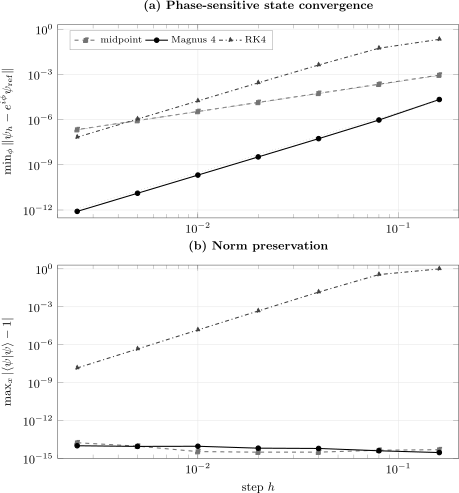

All curves use $\gamma=0.5$ and $X=12$. Panel (a) compares final rays with a Magnus reference at $h=0.0003125$; the thin guides scale as $h^2$ and $h^4$. Panel (b) shows that midpoint and Magnus remain unitary to roundoff, whereas coarse RK4 loses norm and stability. Unitarity and accuracy are distinct tests.

The refined finite-window reference probability is

$$P_{12}^{\mathrm{ref}} = 0.0431911677214.$$

For comparison,

$$P_{\mathrm{LZ}}(0.5) = 0.0432139182638.$$

The finite-window difference is $2.28\times10^{-5}$, much larger than the retained integration error.

$h$	midpoint $\epsilon_\psi$	Magnus $\epsilon_\psi$	RK4 $\epsilon_\psi$	RK4 $\epsilon_N$
$0.16$	$8.93\times10^{-4}$	$2.14\times10^{-5}$	$2.10\times10^{-1}$	$1.00$
$0.08$	$2.21\times10^{-4}$	$9.36\times10^{-7}$	$5.41\times10^{-2}$	$3.54\times10^{-1}$
$0.04$	$5.52\times10^{-5}$	$5.43\times10^{-8}$	$4.16\times10^{-3}$	$1.45\times10^{-2}$
$0.02$	$1.38\times10^{-5}$	$3.33\times10^{-9}$	$2.73\times10^{-4}$	$4.66\times10^{-4}$
$0.01$	$3.45\times10^{-6}$	$2.07\times10^{-10}$	$1.72\times10^{-5}$	$1.46\times10^{-5}$
$0.005$	$8.62\times10^{-7}$	$1.30\times10^{-11}$	$1.08\times10^{-6}$	$4.57\times10^{-7}$
$0.0025$	$2.15\times10^{-7}$	$8.10\times10^{-13}$	$6.76\times10^{-8}$	$1.43\times10^{-8}$

The median observed orders from the asymptotic part of the sweep are

$$\begin{aligned} p_{\mathrm{midpoint}}&=2.0000, \\ p_{\mathrm{Magnus}}&=4.0018, \\ p_{\mathrm{RK4}}&=3.9958. \end{aligned}$$

The unitary methods have maximum norm errors below $1.74\times10^{-14}$ across this sweep. Yet midpoint at $h=0.16$ is about forty times less accurate in state space than fourth-order Magnus while preserving norm equally well. Structure preservation prevents one class of failure; it does not remove truncation error.

RK4 illustrates the complementary warning. At $h=0.16$, its maximum norm error is $0.999985$, so the state is almost extinguished by numerical instability. By $h=0.0025$, fourth-order state convergence is visible, but the norm drift $1.43\times10^{-8}$ is still six orders of magnitude larger than the Magnus state error.

Independent Validation Ledger

Check	Retained value	What it tests
Magnus order	$4.0018$	commutator sign and fourth-order implementation
midpoint order	$2.0000$	independent second-order comparator
RK4 order	$3.9958$	independent right-hand-side implementation
production Magnus step halving	$7.59\times10^{-13}$	state-level integration error at $\gamma=0.5$, $X=12$
largest unitary norm drift in method sweep	$1.73\times10^{-14}$	exponential-step implementation
$\gamma=0.25$, $X=64$ formula difference	$1.37\times10^{-6}$	approach to the asymptotic target
coarse-RK4 norm drift	$0.999985$	stability diagnostic is active
probability bounds	all values in $[0,1]$	observable assembly

These checks are complementary. The Magnus and midpoint norm tests share the same Pauli-exponential helper, so they are not independent validations of that helper. RK4 supplies an independently coded evolution equation, while the analytic probability supplies an asymptotic physical benchmark. The finite-window reference remains numerical; an exact finite-duration parabolic-cylinder solution would provide an additional independent check.

Error Budget at the Representative Point

Take $\gamma=0.5$, $X=12$, and $h=0.0025$.

Source	Retained scale	Interpretation
asymptotic replacement	$2.28\times10^{-5}$ in probability	finite $X$ versus $P_{\mathrm{LZ}}$
Magnus time step	$7.59\times10^{-13}$ in state distance	production versus halved step
Magnus norm drift	below $1.0\times10^{-14}$	accumulated roundoff
endpoint basis protocol	problem-dependent, not an error bar	different preparation and measurement
model discrepancy	not tested	extra levels, nonlinear sweep, and environment absent

The first row dominates the numerical comparison with the infinite-sweep formula. The last row is outside this computation: agreement with Landau–Zener theory does not validate a two-level reduction for a particular experiment.

Reproduce the Calculation

Extract the complete package linked above, then run its entry point from the extracted directory:

python run.py --output-dir results

NumPy is the only required package. The optional —plot flag uses Matplotlib to generate quick-look PNGs from the retained CSV data. The documentation figures use the linked pgfplots sources.

Artifact	Contents
Python program	propagators, sweeps, validation, and data export
window sweep	three couplings, twelve endpoint windows, and two basis protocols
coupling sweep	formula comparison at $X=64$
trajectory	diabatic and adiabatic populations, phase, and norm
integrator convergence	state, probability, and norm errors for three methods
dynamics/window figure source	pgfplots source for the trajectory and endpoint sweep
integrator figure source	pgfplots source for convergence and norm drift

Retained run metadata

Item	Value
run date	2026-07-16
Python	3.12.13
NumPy	2.3.5
arithmetic	binary64 complex amplitudes
random seed	not applicable; no random sampling
wall time on retained machine	$35.7\ \mathrm{s}$
program license	MIT
figure data	direct, unfiltered CSV output

Runtime is hardware-dependent and is not a validation target. Reproduction should compare retained values and the program’s embedded checks.

Algorithm Audit

The implementation follows a short, inspectable sequence.

1. Construct the exact lower instantaneous eigenvector at $x=-X$.
2. Choose an integer number of steps and adjust $h$ so the final point is exactly $+X$.
3. Apply Magnus, midpoint, or RK4 steps while recording the maximum norm deviation.
4. Project onto the exact upper instantaneous eigenvector at $+X$.
5. Repeat from the bare diabatic state and project in the bare basis.
6. Vary $h$ at fixed $X$ for integration convergence.
7. Vary $X$ at fixed small $h$ for endpoint convergence.
8. Compare full final rays with a refined finite-window reference.

No interpolation is used in the endpoint projection. Trajectory samples are diagnostic output only and do not feed back into the propagation.

Known Failure Modes

• Changing the Hamiltonian convention: if the diagonal entries, coupling, or sweep slope are renamed, the exponent and dimensionless equation must be translated together.
• Bare-state preparation at finite detuning: $\lvert1\rangle$ is not exactly $\lvert-;-X\rangle$. The resulting difference is coherent and need not decrease monotonically.
• One-window confirmation: an accidental cancellation can make one $X$ look converged. Test an envelope over several larger windows.
• One-step confirmation: agreement after halving $h$ says nothing about finite-endpoint error.
• Coarse RK4 at large detuning: the endpoint oscillation frequency grows with $\gamma X$ and can leave the RK4 stability region.
• Renormalizing every RK4 step: forced normalization hides norm loss but does not repair relative-phase or population error.
• Treating unitarity as accuracy: exponential midpoint preserves norm exactly while retaining second-order state error.
• Probability-only convergence: one scalar can converge through cancellation while the final ray remains inaccurate.
• Tiny probabilities: for large $\gamma$, relative errors become sensitive to underflow and absolute roundoff. Logarithmic formulations or exact asymptotics may be needed.
• Adaptive steps without a physical audit: a local tolerance does not automatically control the final transition probability or finite-window error.
• Repeated passages: two crossings produce Stückelberg interference and require a phase-aware multi-passage calculation.
• Open-system dynamics: relaxation, dephasing, and noise require a density-matrix or stochastic model; a norm-preserving spinor solver cannot represent them.
• More than two levels: an apparently isolated avoided crossing can be contaminated by nearby states even when this two-level computation is perfectly converged.
• Nonlinear or truncated ramps: the ideal exponent need not remain exact when detuning is nonlinear or coupling is time-dependent.

Further Investigations

1. Implement the exact finite-duration solution with parabolic-cylinder functions and compare it directly with the numerical $P_X$.
2. Use a symmetric nonlinear sweep and identify which local slope, if any, controls an effective Landau–Zener exponent.
3. Add a second passage and recover Stückelberg fringes as a function of waiting phase.
4. Propagate a Lindblad master equation and separate dephasing from endpoint error.
5. Compare fixed-step Magnus with an adaptive commutator-free exponential integrator.
6. Repeat the state-error audit in a moving adiabatic basis and track the geometric connection explicitly.

Exercises

Nondimensionalize the equation

Starting from

$$i\hbar\frac{d\psi}{dt} = \left( \frac{vt}{2}\sigma_z + \Delta\sigma_x \right)\psi,$$

derive the dimensionless equation used by the program.

Solution

Set $x=vt/(2\Delta)$, so

$$\frac{d}{dt} = \frac{v}{2\Delta} \frac{d}{dx}.$$

Also $vt/2=\Delta x$. Substitution gives

$$i\hbar \frac{v}{2\Delta} \frac{d\psi}{dx} = \Delta \left(x\sigma_z+\sigma_x\right)\psi.$$

Multiplying by $2\Delta/(\hbar v)$ and defining $\gamma=\Delta^2/(\hbar v)$ yields

$$i\frac{d\psi}{dx} = 2\gamma \left(x\sigma_z+\sigma_x\right)\psi.$$

Recover the Magnus commutator term

For the two Gauss nodes, show that the fourth-order exponent contains

$$-i\frac{2}{3}\gamma^2h^3\sigma_y.$$

Solution

Let $B(x)=x\sigma_z+\sigma_x$, so $A(x)=-2i\gamma B(x)$. Using

$$[\sigma_z,\sigma_x] = 2i\sigma_y,$$

one finds

$$\begin{aligned} [B(x_1),B(x_2)] &= 2i(x_1-x_2)\sigma_y \\ &= -\frac{2i\sqrt3}{3}h\,\sigma_y. \end{aligned}$$

Therefore

$$[A_1,A_2] = \frac{8i\sqrt3}{3} \gamma^2h\,\sigma_y.$$

Multiplying by the Magnus coefficient gives

$$-\frac{\sqrt3h^2}{12}[A_1,A_2] = -i\frac{2}{3}\gamma^2h^3\sigma_y.$$

Together with the averaged generator, this is $\Omega_4=-iK$ with the $K$ stated above.

Estimate the observed order

Use the Magnus state errors at $h=0.04$ and $h=0.02$ to estimate the convergence order.

Solution

For step halving,

$$p_{\mathrm{obs}} = \frac{ \log(\epsilon_{0.04}/\epsilon_{0.02}) }{ \log2 }.$$

Using $5.429\times10^{-8}$ and $3.334\times10^{-9}$ gives

$$p_{\mathrm{obs}} \approx \frac{\log(16.28)}{\log2} \approx4.03.$$

Later pairs approach $4$ more closely. The deviation here reflects pre-asymptotic contributions and the finite numerical reference.

Separate endpoint and integration error

At $\gamma=0.5$ and $X=12$, the production state changes by $7.59\times10^{-13}$ under step halving, but the probability differs from $P_{\mathrm{LZ}}$ by $2.28\times10^{-5}$. What conclusion is justified, and what conclusion is not?

Solution

The justified conclusion is that time-step error is negligible relative to the discrepancy with the infinite-sweep formula. The natural remaining numerical explanation is the finite endpoint $X=12$, which should be tested by increasing $X$ while maintaining step resolution.

It is not justified to claim that the underlying two-level model describes a laboratory system to $2.28\times10^{-5}$. Extra levels, ramp nonlinearity, decoherence, and parameter uncertainty are model errors absent from this calculation.

Explain why norm is insufficient

At $h=0.16$, both midpoint and Magnus preserve norm to about $10^{-15}$, yet their phase-aligned state errors are $8.93\times10^{-4}$ and $2.14\times10^{-5}$. Why is there no contradiction?

Solution

Norm preservation constrains the state to remain on the unit sphere. It does not determine where on that sphere the state lies. A unitary approximation can rotate by the wrong angle or around the wrong axis while preserving norm exactly.

Magnus includes the leading noncommutativity correction and is fourth order. Exponential midpoint omits that term and is second order. Both are unitary, but their trajectory errors differ.

Design an endpoint stopping rule

Why is the criterion $|P_{2X}-P_X|<\varepsilon$ at one pair of windows unsafe here? Propose a stronger rule.

Solution

The endpoint error oscillates because small amplitudes generated near the boundaries acquire changing dynamical phases. Two neighboring windows can agree through accidental cancellation even when the envelope remains larger than $\varepsilon$.

A stronger empirical rule evaluates several increasing windows, such as $X$, $1.25X$, $1.5X$, and $2X$, and requires all pairwise changes from the largest-window result to remain below the tolerance. It should be repeated after step refinement because the endpoint frequency grows with $X$. When available, comparison with an exact finite-duration solution is stronger still.

Cross-Links

• Computational Notebooks
• Landau–Zener Transition
• Landau–Zener Transition Worked Example
• Landau–Zener Problem: First Encounter
• Adiabatic Approximation
• Sudden Approximation
• Time-Dependent Hamiltonians
• Unitary Time Evolution
• ODE Solvers
• Convergence Tests

References

• L. D. Landau, “Zur Theorie der Energieübertragung. II,” Physikalische Zeitschrift der Sowjetunion 2, 46–51 (1932).
• C. Zener, “Non-Adiabatic Crossing of Energy Levels,” Proceedings of the Royal Society A 137, 696–702 (1932), doi:10.1098/rspa.1932.0165.
• E. Majorana, “Atomi orientati in campo magnetico variabile,” Il Nuovo Cimento 9, 43–50 (1932), doi:10.1007/BF02960953.
• N. V. Vitanov and B. M. Garraway, “Landau–Zener model: Effects of finite coupling duration,” Physical Review A 53, 4288–4304 (1996), doi:10.1103/PhysRevA.53.4288.
• S. N. Shevchenko, S. Ashhab, and F. Nori, “Landau–Zener–Stückelberg interferometry,” Physics Reports 492, 1–30 (2010), doi:10.1016/j.physrep.2010.03.002.
• W. Magnus, “On the exponential solution of differential equations for a linear operator,” Communications on Pure and Applied Mathematics 7, 649–673 (1954), doi:10.1002/cpa.3160070404.
• S. Blanes, F. Casas, J. A. Oteo, and J. Ros, “The Magnus expansion and some of its applications,” Physics Reports 470, 151–238 (2009), doi:10.1016/j.physrep.2008.11.001.
• E. Hairer, C. Lubich, and G. Wanner, Geometric Numerical Integration: Structure-Preserving Algorithms for Ordinary Differential Equations, 2nd ed., Springer, 2006.